28 April 2020, Tuesday
In this note, we derive localised approximations to the hyperbolic tangent.
In machine learning, activation functions squash a real value to another real value in a specified range. When the range is \([-1, 1]\), one could use the hyperbolic tangent (denoted as \(\tanh\)). For instance, hyperbolic tangents are prominent components of Long Short-Term Memory (LSTM) form of Recurrent Neural Networks (RNN).
Johann Heinrich Lambert (1728–1777) gave use the exponential expression of the hyperbolic tangent:
\[ \begin{equation} \tanh x = \frac{\sinh x}{\cosh x} = \frac {e^x - e^{-x}} {e^x + e^{-x}} = \frac{e^{2x} - 1} {e^{2x} + 1}. \label{eqn:tanh expressions} \end{equation} \]
In the following, we provide three derivations for localised approximations of \(\tanh\) and provide a SIMD implementation.
On the history of hyperbolic functions, see J. H. Barnett, “Enter, Stage Center: The Early Drama of the Hyperbolic Functions,” Mathematics Magazine, vol. 77, no. 1, pp. 15–30, 2004. Hyperbolic functions were first studied by Vincenzo Riccati (1707–1775) to solve cubic equations. The current notation for hyperbolic functions, for instance, \(\tanh\) for the hyperbolic tangent, were first used by Johann Heinrich Lambert [See page 71 of James McMahon, “Hyperbolic Functions,” Fourth Edition, John Wiley & Sons, 1906].
In 1770, Johann Heinrich Lambert first developed the process for reducing the quotient of two convergent series into continued fractions [See page 75 in J. H. Lambert, “Beyträge zum Gebrauche der Mathematik und deren Anwendung (Contributions to the use of Mathematics and its Application),” vol. II. Berlin: Verlag der Buchhandlung der Realschule, 1770]. Using this process, we can express the hyperbolic tangent as follows:
\[\begin{align} \tanh x = \frac{x}{1 + \cfrac{x^2}{3 + \cfrac{x^2}{5 + \cfrac{x^2}{7 + \ddots}}}}. \end{align}\]
This is referred to as Lambert’s continued fraction. The following is the 7th-degree Lambert approximant for \(\tanh\):
\[\begin{align} \tanh x \approx \frac{135135x + 17325x^3 + 378x^5 + x^7}{135135 + 62370 x^2 + 3150x^4 + 28 x^6}.\label{eqn:7-th degree lambert approximant} \end{align}\]
Although Lambert did not explicitly give the derivation of \(\tanh\), we can derive it using his method for continued fractions [See pages 517–522 in G. Chrystal, “Algebra: An Elementary Text-Book for the Higher Classes of Secondary Schools and for Colleges,” vol. II. London: Adam and Charles Black, 2nd ed., 1900. First published 1889]. We shall present a derivation here, as it is interesting.
Let \(f_0, f_1, f_2, \ldots\) be a sequence of analytic functions defined for an independent variable \(z\). Analytic functions are functions locally defined by a power series. For instance, the hyperbolic sine and cosine are defined by the Taylor series:
\[\begin{align} \sinh x &= x + \frac {x^3} {3!} + \frac {x^5} {5!} + \frac {x^7} {7!} +\cdots = \sum_{n=0}^\infty \frac{x^{2n+1}}{(2n+1)!},\label{eqn:sinh series}\\ \cosh x &= 1 + \frac {x^2} {2!} + \frac {x^4} {4!} + \frac {x^6} {6!} + \cdots = \sum_{n=0}^\infty \frac{x^{2n}}{(2n)!}. \label{eqn:cosh series} \end{align}\]
If \(f_{i - 1} - f_{i} = k_izf_{i+1}\) for all \(i > 0\), where \(k_i\) is a constant, then
\[\begin{align} \cfrac{f_{i-1}}{f_i} = 1 + \cfrac{k_izf_{i+1}}{f_i}{\rm;\ or,\ }\cfrac{f_i}{f_{i-1}} = \cfrac{1}{1 + \cfrac{k_izf_{i+1}}{f_i}}. \label{eqn:frac f_i f_i-1} \end{align}\]
If we define \(g_i\) as \(\dfrac{f_i}{f_{i-1}}\), then \(\eqref{eqn:frac f_i f_i-1}\) can be expressed as:
\[\begin{align} g_i = \cfrac{1}{1 + k_izg_{i+1}}\nonumber \end{align}\]
from which we get the continued fractions
\[\begin{align} g_1 = \frac{f_1}{f_0} = \cfrac{1}{1 + k_1zg_{2}} = \cfrac{1}{1 + \cfrac{k_1z}{1 + k_2zg_{3}}} = \cfrac{1}{1 + \cfrac{k_1z}{1 + \cfrac{k_2z}{1 + k_3zg_{4}}}}\textrm{, and so on.} \label{eqn:continued fractions expansion} \end{align}\]
Let \(F(a;z)\) be an analytic function on \(z\) parametrised by constant \(a\), such that
\[\begin{align} F(a;z) = 1 + \frac{1}{a}\cdot\frac{z}{1!} + \frac{1}{a(a+1)}\cdot\frac{z^2}{2!} + \frac{1}{a(a+1)(a+2)}\cdot\frac{z^3}{3!} + \cdots. \label{eqn:series 0f1} \end{align}\]
From this, we get
\[\begin{align} F(a-1;z) - F(a;z) &=\left[\frac{1}{(a-1)}-\frac{1}{a}\right]\frac{z}{1!} + \left[\frac{1}{(a-1)a}-\frac{1}{a(a+1)}\right]\frac{z^2}{2!} + \cdots\nonumber\\ &= \frac{z}{a(a-1)}\left[1 + \frac{1}{(a+1)}\cdot\frac{z}{1!} + \cdots\right]\nonumber\\ &= \frac{z}{a(a-1)}\,F(a+1;z). \label{eqn:series subtraction} \end{align}\]
If we let \(f_i = F(a+i;z)\) and \(k_i = \dfrac{1}{(a+i)(a+i-1)}\) then \(\eqref{eqn:series subtraction}\) can be written as \(f_{i-1} - f_i = k_izf_{i+1}\). This means we can use \(\eqref{eqn:continued fractions expansion}\) to get
\[\begin{align} g_1 = \frac{f_1}{f_0} &= \cfrac{1}{1 + \cfrac{\cfrac{z}{(a+1)a}}{1 + \cfrac{\cfrac{z}{(a+2)(a+1)}}{1 + \cfrac{z}{(a+3)(a+2)}\cdot g_{4}}}}\nonumber \end{align}\]
so that
\[\begin{align} \frac{f_1}{f_0} &= \cfrac{a}{a + \cfrac{z}{(a+1) + \cfrac{z}{(a+2) + \cfrac{z}{(a+3) + \ddots}}}}. \label{eqn:f_1f_0 continued fractions} \end{align}\]
Now, using the function \(F\) defined in \(\eqref{eqn:series 0f1}\), we can write the hyperbolic sine and cosine functions expressed in \(\eqref{eqn:sinh series}\) and \(\eqref{eqn:cosh series}\) as \(xF(3/2;x^2/4)\) and \(F(1/2;x^2/4)\) respectively. Thus,
\[\begin{align} \tanh x = \frac{\sinh x}{\cosh x} = \frac{xF(3/2;x^2/4)}{F(1/2;x^2/4)} = \frac{xF(a+1;z)}{F(a;z)} = x\cdot\frac{f_1}{f_0} \end{align}\]
where, \(a = 1/2\) and \(z = x^2/4\). Substituting these in \(\eqref{eqn:f_1f_0 continued fractions}\) we get
\[\begin{align} \tanh x = x\cdot\cfrac{1/2}{\cfrac{1}{2} + \cfrac{x^2/4}{\left(\cfrac{1}{2}+1\right) + \cfrac{x^2/4}{\left(\cfrac{1}{2}+2\right) + \cfrac{x^2/4}{\left(\cfrac{1}{2}+3\right) + \ddots}}}} = \frac{x}{1 + \cfrac{x^2}{3 + \cfrac{x^2}{5 + \cfrac{x^2}{7 + \ddots}}}}.\nonumber \end{align}\]
Johann Carl Friedrich Gauss (1777–1855) systematised the study of continued fractions [See pages 134–138 of J. C. F. Gauss, “Werke (Works),” vol. III. Göttingen: Königlichen Gesellschaft der Wissenschaften (Royal Society of Sciences), 2nd ed., 1876. First published 1866] and provided a general method for reducing quotient of convergent series to continued fractions. This method can be used for deriving continued fractions of various functions that are used in machine learning, for instance the exponential function \(\exp(x)\) [Ibid, pages 127 and 136].
Another representation of the hyperbolic tangent as a power series [See page 343 in G. Chrystal, “Algebra: An Elementary Text-Book for the Higher Classes of Secondary Schools and for Colleges,” vol. II. London: Adam and Charles Black, 2nd ed., 1900. First published 1889] is given as:
\[\begin{align} \tanh x = \sum_{n=1}^\infty\frac{(-1)^{n-1}2^{2n}(2^{2n}-1)B_{n}x^{2n-1}}{(2n)!} \label{eqn:tanh bernoulli} \end{align}\]
where, \(B_{n}\) is a Bernoulli number defined [ Ibid, page 231] as follows:
\[\begin{align} (-1)^{n-1}n = \sum_{i=1}^{n}(-1)^{n-i}\binom{2n+2}{2i}B_i. \end{align}\]
Substituting \(n = 1, 2, 3, \ldots\) we have,
\[\begin{align} (-1)^{1-1}1 &= (-1)^{1-1}\binom{2\times1+2}{2}B_1 = \binom{4}{2}B_1\textrm{, giving}B_1 = \frac{1}{6};\nonumber\\ (-1)^{2-1}2 &= (-1)^{2-1}\binom{2\times2+2}{2\times1}B_1 + (-1)^{2-2}\binom{2\times2+2}{2\times2}B_2\nonumber\\ &= -1\times\binom{6}{2}\frac{1}{6} + \binom{6}{4}B_2\textrm{, giving }B_2 = \frac{1}{30};\nonumber\\ B_3 &= \frac{1}{42}, B_4 = \frac{1}{30}\textrm{, and so on.}\nonumber \end{align}\]
Substituting these in \(\eqref{eqn:tanh bernoulli}\), we get
\[\begin{align} \tanh x = x - \frac {x^3} {3} + \frac {2x^5} {15} - \frac {17x^7} {315} + \cdots \end{align}\]
Another approximation of the hyperbolic tangent can be defined using the Padé approximation of the exponential function. The following is a \([5/5]\) Padé approximant of \(\exp()\):
\[\begin{equation} \exp(x) \approx \frac{1 + \dfrac{1}{2}x + \dfrac{1}{9}x^2 + \dfrac{1}{72}x^3 + \dfrac{1}{1008}x^4 + \dfrac{1}{30240}x^5}{1 - \dfrac{1}{2}x + \dfrac{1}{9}x^2 - \dfrac{1}{72}x^3 + \dfrac{1}{1008}x^4 - \dfrac{1}{30240}x^5}. \end{equation}\]
Hence,
\[\begin{equation} \exp(2x) \approx \frac{1 + x + \dfrac{4}{9}x^2 + \dfrac{1}{9}x^3 + \dfrac{1}{63}x^4 + \dfrac{1}{945}x^5}{1 - x + \dfrac{4}{9}x^2 - \dfrac{1}{9}x^3 + \dfrac{1}{63}x^4 - \dfrac{1}{945}x^5}. \end{equation}\]
From \(\eqref{eqn:tanh expressions}\), \(\tanh(x) = \dfrac{e^{2x} - 1}{e^{2x} + 1}\); hence:
\[\begin{equation} \tanh(x) \approx \frac{945x + 105x^3+ x^5}{945 + 420x^2 + 15x^4}. \end{equation}\]
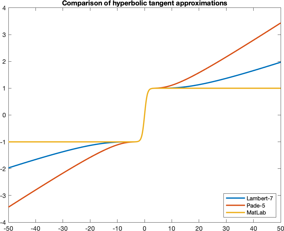
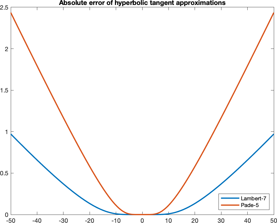
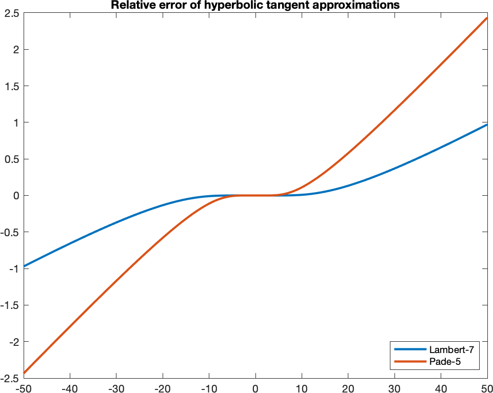
The following shows a comparison of hyperbolic tangent approximations using Lambert-9 and Padé \([5/5]\) approximant. This shows that we need to clamp the values to lie in the interval \([-1, 1]\).
Sequential implementation of hyperbolic tanget. The function is passed parameters r and m, which are valid memory pointers that point to buffers that can accommodate at least n floating-point values. Buffer m contains the original n values (i.e., the values of x), and buffer r is where the results of tanh(x) are stored.
<Functions>+=
void af_tanh_seq(float *r, float const *m, size_t n)
{
    for (size_t i = n; i; --i) {
        *r++ = tanhf(*m++);
    }
}The Short Vector Math Library (SVML) instruction set is only available through Intel C++ Compiler (ICC) and proprietary library. If this is unavailable, implement the vectorised approximation using Lambert’s continued fractions.
Applying Horner’s scheme for efficient evaluation of polynomials to \(\eqref{eqn:7-th degree lambert approximant}\), we get:
\[\begin{align} \tanh(x) \approx \frac{x(135135 + x^2(17325 + x^2(378 + x^2)))}{135135 + x^2(62370 + x^2(3150 + 28x^2))}. \end{align}\]
In the following, we implement this using SIMD intrinsics.
<Functions>+=
#if !defined(__INTEL_COMPILER)
#if defined(__SSE__)
    <Implement tanh() using SSE>
#endif
#if defined(__AVX__)
    <Implement tanh() using AVX>
#endif
#if defined(__AVX512F__)
    <Implement tanh() using AVX512F>
#endif
#endif /* #if !defined(__INTEL_COMPILER) */
Implement tanh() using SSE intrinsics.
<Implement tanh() using SSE>=
__m128 _mm_tanh_ps(__m128 x)
{
    __m128 xs = _mm_mul_ps(x, x);
    __m128 n = _mm_add_ps(xs, _mm_set1_ps(378));
    n = _mm_mul_ps(n, xs);
    n = _mm_add_ps(n, _mm_set1_ps(17325));
    n = _mm_mul_ps(n, xs);
    n = _mm_add_ps(n, _mm_set1_ps(135135));
    n = _mm_mul_ps(n, x);

    __m128 d = _mm_mul_ps(xs, _mm_set1_ps(28));
    d = _mm_add_ps(d, _mm_set1_ps(3150));
    d = _mm_mul_ps(d, xs);
    d = _mm_add_ps(d, _mm_set1_ps(62370));
    d = _mm_mul_ps(d, xs);
    d = _mm_add_ps(d, _mm_set1_ps(135135));

    n = _mm_div_ps(n, d);
    n = _mm_min_ps(n, _mm_set1_ps(1));
    n = _mm_max_ps(n, _mm_set1_ps(-1));
    return n;
}
Implement tanh() using AVX intrinsics.
<Implement tanh() using AVX>=
__m256 _mm256_tanh_ps(__m256 x)
{
    __m256 xs = _mm256_mul_ps(x, x);
    __m256 n = _mm256_add_ps(xs, _mm256_set1_ps(378));
    n = _mm256_mul_ps(n, xs);
    n = _mm256_add_ps(n, _mm256_set1_ps(17325));
    n = _mm256_mul_ps(n, xs);
    n = _mm256_add_ps(n, _mm256_set1_ps(135135));
    n = _mm256_mul_ps(n, x);

    __m256 d = _mm256_mul_ps(xs, _mm256_set1_ps(28));
    d = _mm256_add_ps(d, _mm256_set1_ps(3150));
    d = _mm256_mul_ps(d, xs);
    d = _mm256_add_ps(d, _mm256_set1_ps(62370));
    d = _mm256_mul_ps(d, xs);
    d = _mm256_add_ps(d, _mm256_set1_ps(135135));

    n = _mm256_div_ps(n, d);
    n = _mm256_min_ps(n, _mm256_set1_ps(1));
    n = _mm256_max_ps(n, _mm256_set1_ps(-1));
    return n;
}
Implement tanh() using AVX512 intrinsics.
<Implement tanh() using AVX512F>=
__m512 _mm512_tanh_ps(__m512 x)
{
    __m512 xs = _mm512_mul_ps(x, x);
    __m512 n = _mm512_add_ps(xs, _mm512_set1_ps(378));
    n = _mm512_mul_ps(n, xs);
    n = _mm512_add_ps(n, _mm512_set1_ps(17325));
    n = _mm512_mul_ps(n, xs);
    n = _mm512_add_ps(n, _mm512_set1_ps(135135));
    n = _mm512_mul_ps(n, x);

    __m512 d = _mm512_mul_ps(xs, _mm512_set1_ps(28));
    d = _mm512_add_ps(d, _mm512_set1_ps(3150));
    d = _mm512_mul_ps(d, xs);
    d = _mm512_add_ps(d, _mm512_set1_ps(62370));
    d = _mm512_mul_ps(d, xs);
    d = _mm512_add_ps(d, _mm512_set1_ps(135135));

    n = _mm512_div_ps(n, d);
    n = _mm512_min_ps(n, _mm512_set1_ps(1));
    n = _mm512_max_ps(n, _mm512_set1_ps(-1));
    return n;
}If instructions are available, process four at a time. Note how we cascade to sequential implementation when the number of values to process is less than 4.
<Functions>+=
#if defined(__SSE__)
void af_tanh_sse(float *r, float const *m, size_t n)
{
    if (n == 0) {
        return;
    }
    size_t l = n % 4;
    n -= l;
    if (n) {
        while (n) {
            __m128 x = _mm_loadu_ps(m);
            x = _mm_tanh_ps(x);
            _mm_storeu_ps(r, x);
            m += 4;
            r += 4;
            n -= 4;
        }
    }
    if (l) {
        af_tanh_seq(r, m, l);
    }
}
#endif /* #if defined(__SSE__) */If instructions are available, process eight at a time. Note how we cascade to narrow implementation when the number of values to process is less than 8. This is possible because availability of wider SIMD instructions also means availability of narrower SIMD instructions.
<Functions>+=
#if defined(__AVX__)
void af_tanh_avx(float *r, float const *m, size_t n)
{
    if (n == 0) {
        return;
    }
    size_t l = n % 8;
    n -= l;
    if (n) {
        while (n) {
            __m256 v = _mm256_loadu_ps(m);
            v = _mm256_tanh_ps(v);
            _mm256_storeu_ps(r, v);
            m += 8;
            r += 8;
            n -= 8;
        }
    }
    if (l) {
        af_tanh_sse(r, m, l);
    }
}
#endif /* #if defined(__AVX__) */If instructions are available, process sixteen at a time. Note how we cascade to implementation when the number of values to process is less than 16.
<Functions>+=
#if defined(__AVX512F__)
void af_tanh_avx512f(float *r, float const *m, size_t n)
{
    if (n == 0) {
        return;
    }
    size_t l = n % 16;
    n -= l;
    if (n) {
        while (n) {
            __m512 v = _mm512_loadu_ps(m);
            v = _mm512_tanh_ps(v);
            _mm512_storeu_ps(r, v);
            m += 16;
            r += 16;
            n -= 16;
        }
    }
    if (l) {
        af_tanh_avx(r, m, l);
    }
}
#endif /* #if defined(__AVX512F__) */To apply hyperbolic tangent activation on a list of values, programs should only use the following interface. This invokes the best implementation depending on the availability of SIMD instructions, choosing the widest instruction when possible.
<Functions>+=
void af_tanh(float *r, float const *m, size_t n)
{
#if defined(__AVX512F__)
    af_tanh_avx512f(r, m, n);
#elif defined(__AVX__)
    af_tanh_avx(r, m, n);
#elif defined(__SSE__)
    af_tanh_sse(r, m, n);
#else
    af_tanh_seq(r, m, n);
#endif
}We test the implementation using a simple example.
<Test functions>+=
void test_tanh()
{
    size_t n = 1000;
    float m[1000], r[1000];
    float l = -5, h = -l, v = l;
    float dx = (h - l)/(n - 1);
    for (size_t i = 0; i < n; ++i) {
        m[i] = v;
        v += dx;
    }
    af_tanh(r, m, n);
    for (size_t i = 0; i < n; ++i) {
        printf("%f -> %f\n", m[i], r[i]);
    }
}
Main program for testing the functions.
<Main>=
int main(void) {
    test_relu();
    test_tanh();
    return 0;
}

<Standard libraries>=
#include <math.h>
#include <stdio.h>
#include <string.h>
#include <immintrin.h>
#include <xmmintrin.h>

<algorithm.c>=
<Standard libraries>
<Functions>
<Test functions>
<Main>