26 May 2020, Tuesday
In this note, we investigate various loop orderings for matrix multiplication and improve cache utilisation based on these orderings. We also provide SIMD implementation of the variants.
Given two matrices \(A\) and \(B\) with respective dimensions \(k \times l\) and \(m \times n\), our objective is to determine the following matrix products efficiently: 1) \(A\times B\), 2) \(A^T\times B\) and 3) \(A\times B^T\); where \(A^T\) denotes the transpose of \(A\). These three types of matrix products are prevalent in machine learning algorithms.
Let us simplify our notation by removing the multiplication symbol, so that \(A\times B\) is denoted simply as \(AB\); \(A^T\times B\) as \(A^TB\), and \(A \times B^T\) as \(AB^T\).
If we denote with \(A_{ij}\) the \(j\)th column element of the \(i\)th row of a matrix \(A\) where \(0 \le i < k\) and \(0 \le j < l\), then \(A_{ij}\) is also the \(i\)th column element of the \(j\)th row of \(A^T\). In other words, the number of rows and columns in \(A\) respectively equals the number of columns and rows in \(A^T\).
By definition, \(l = m\) is the precondition for \(AB\) which produces a matrix \(C\) with dimensions \(k \times n\). Similarly, \(k = m\) is the precondition for \(A^TB\) producing \(C\) with dimensions \(l\times n\); and \(l = n\) for \(AB^T\) producing \(C\) with dimensions \(k\times m\).
While it is tempting to simplify our objectives by first finding an efficient implementation for \(AB\) and then applying the same to \(A^TB\) and \(AB^T\), albeit by first computing the transpose \(A^T\) and \(B^T\) for matrices \(A\) and \(B\) respectively prior to calculating the products, we must know that in-place transposition of a non-square matrix is not simple, and doing transposition using a separate memory for the transpose is expensive due to the additional memory requirement. As we will soon see, the transposition operation is an unnecessary overhead that we can avoid, simply by organising the loops.
What we shall do, therefore, is first to determine an efficient implementation for \(AB\), which we will then adapt to calculate \(A^TB\) and \(AB^T\) by simply modifying the array indexing pattern.
An \(m\times n\) matrix can be stored in memory as a one-dimensional array of length \((m \times n)\). This is achieved using one of two memory storage conventions. The first is the row-major form, where all column elements of a given row are stored in sequence so that they occupy sequential addresses in memory. The second is the column-major form where all row elements of a given column are stored in sequence. The following is an example of the two conventions:

We shall use the row-major form in the following discussions.
Given two matrices \(A\) and \(B\) with respective dimensions \(l \times m\) and \(m \times n\), where the matrix elements have been stored in memory using row-major form, a naïve implementation of the matrix multiplication algorithm that produces \(C = AB\) can be expressed as follows:
void matmul_ijk(
    float *C, const float *A, const float *B,
    size_t l, size_t m, size_t n)
{
    for (size_t i = 0; i < l; ++i) {
        for (size_t j = 0; j < n; ++j) {
            register const float *a = A;
            register const float *b = B + j;
            register float s = 0.0;
            for (size_t k = 0; k < m; ++k) {
                s += *a++ * *b;
                b += n;
            }
            *C++ = s;
        }
        A += m;
    }
}
Why is this implementation considered naïve? Actually, if the microprocessor cache was large enough to fit all of the matrices \(A\), \(B\) and \(C\), then this implementation is not only simple, but also efficient. However, most of the matrices that we will encounter in machine learning do not fit inside the microprocessor cache, as the cache is indeed quite a limited resource. Therefore, when the size of the matrices are larger than the available cache, the above algorithm manifests serious performance bottlenecks as out-of-cache access is computationally very expensive. To understand why this is so, we must look at the memory access pattern of this algorithm, which determines its cache utilisation behaviour.
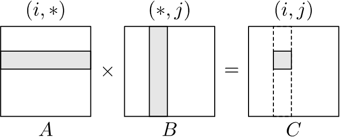
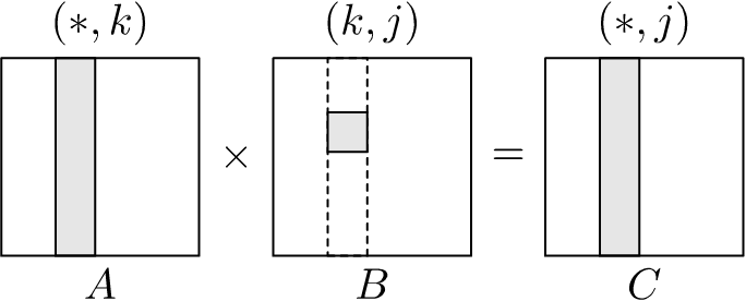
Since it is easier to depict the memory access pattern of a matrix multiplication algorithm visually rather than attempt to describe it using only words, we shall use a graphical representation. Figure 1.1 shows the memory access pattern for matmul_ijk(). It depicts the access pattern where the innermost \(k\)-loop iterates through all column elements of the \(i\)th row in matrix \(A\) moving left to right, while also iterating over all row elements on the \(j\)th column in matrix \(B\) moving top to bottom. These are denoted respectively as \((i, *)\) and \((*, j)\), which correspond to the shaded row and column on matrices \(A\) and \(B\).

We run the \(k\)-loop for each iteration of the \(j\)-loop, which in turn is repeated for each iteration of the \(i\)-loop. The dotted row in \(C\) means the \(j\)-loop is run for the current iteration of the \(i\)-loop; and the shaded region in \(C\) represents the element of the product at the \(j\)th column of the \(i\)th row that will be calculated at the end of the current \(k\)-loop. Hence, with every completed iteration of the \(k\)-loop, we obtain a final element of \(C\).
-’ denote values not in \(A\).If the matrix elements are stored using row-major form, the two access patterns \((i, *)\) and \((*, j)\) have different performance characteristics.
With the \((i, *)\) access pattern, accessing the first element of \(A\) will result in a cache miss (assuming that element is being accessed for the first time). The microprocessor will load the value from memory into the cache using expensive load instructions. While loading this value, however, the microprocessor will also load the next few consecutive elements in the array onto the cache.
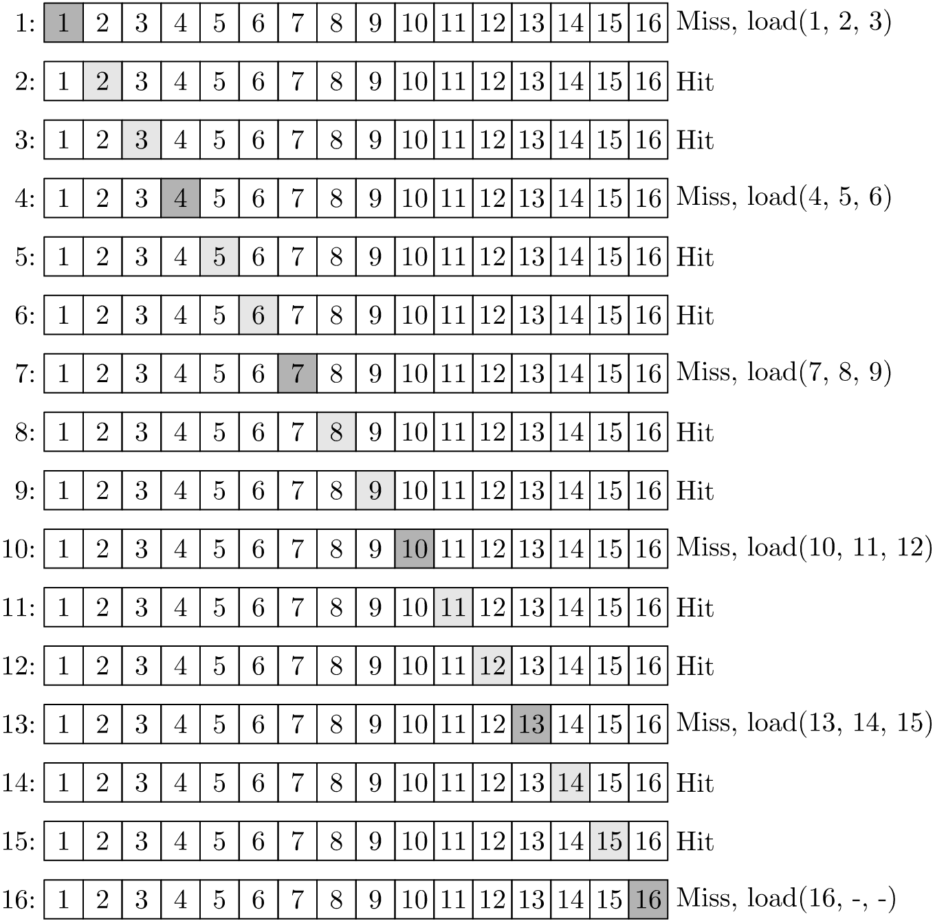
The number of elements that gets loaded into the cache depends on the size of the cache line and the number of available cache lines inside the microprocessor. This means that when the microprocessor accesses the next element of \(A\) in the same row, it will get a cache hit, thus avoiding the expensive memory load instructions. This will continue until the cache is exhausted at which point the microprocessor will get a cache miss, which triggers another memory load. For example, using the \(4\times 4\) matrix shown previously stored in row-major form, and assuming a single cache line that can accommodate upto 3 matrix elements at a time, \((i, *)\) access of \(A\) will incur 6 cache misses and 10 cache hits. This is shown in Figure 1.2.
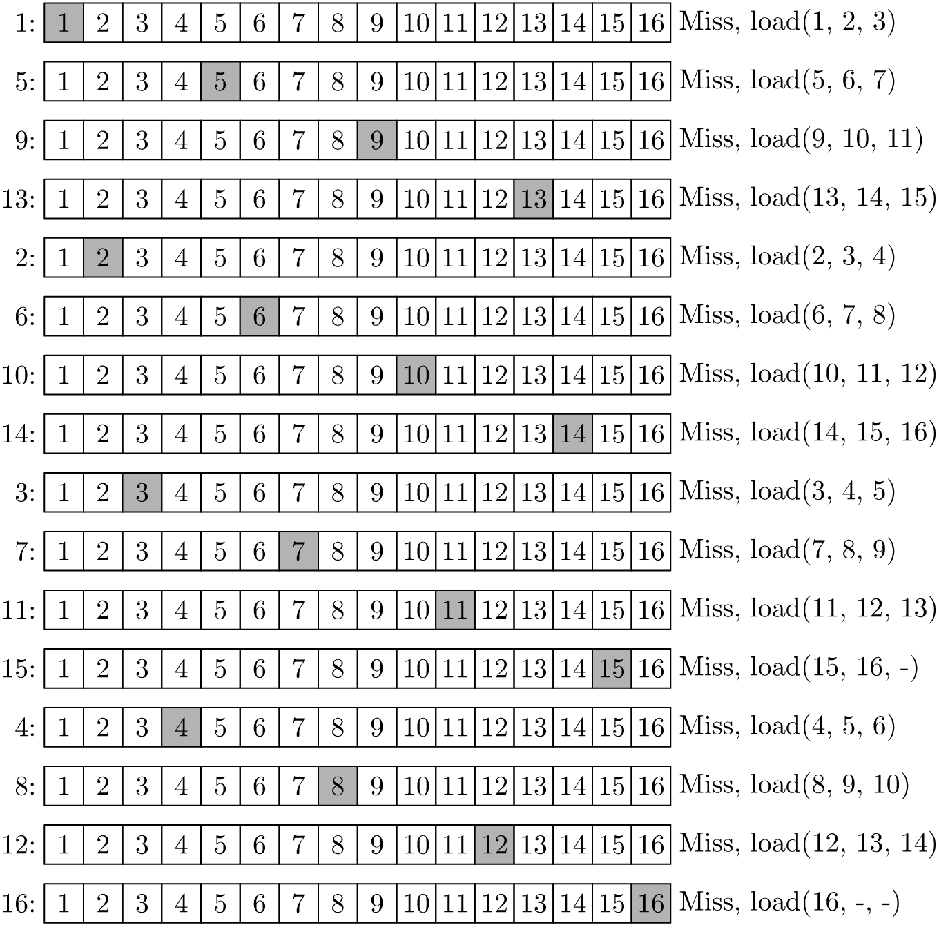
-’ denote values not in \(A\).On the other hand, using the same matrix \(A\) and same cache line capacity, the \((*, j)\) access pattern will incur 16 cache misses and no cache hits. This is because every access to an element results in a miss because the preloaded values in the cache are not all utilised before they are evicted, requiring a load from memory for every element in \(A\). This is shown in Figure 1.3. Hence, the \((*, j)\) pattern is not cache efficient. As a consequence, matrix multiplication using the \(ijk\)-loop ordering is not cache efficient as it uses the \((*, j)\) pattern when accessing elements of \(B\).
Figures 1.4 shows the various memory access patterns that correspond to the six permutations for organising the three loops.
| ijk: |
|
| jik: |
|
| ikj: |
|
| kij: |

|
| jki: |
|
| kji: |

|
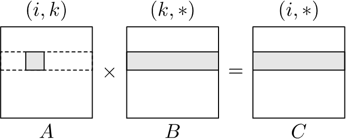
So what are the possible loop orderings for matrix multiplication and what access patterns do they manifest? Are there loop orderings better than \(ijk\)? By ‘better’, we mean orderings that avoid the cache inefficient \((*, j)\) access pattern. In fact, there are two such orderings out of the possible six. These are shown in Figures 1.4. The cache efficient loop orderings are \(ikj\) and \(kij\), of which the better option is the \(ikj\) ordering as it avoids the \((*, j)\) pattern for all three loops.
void matmul_ikj(
    float *C, const float *A, const float *B,
    size_t l, size_t m, size_t n)
{
    <Initialise output matrix to zero>
    register const float *a = A;
    for (size_t i = 0; i < l; ++i) {
        register const float *b = B;
        for (size_t k = 0; k < m; ++k) {
            c = C;
            for (size_t j = 0; j < n; ++j) {
                *c++ += *a * *b++;
            }
            ++a;
        }
        C += n;
    }
}
Notice in Figures 1.4 that for all loop orderings where the dotted rows and columns exist in the product matrix \(C\), each completed iteration of the innermost loop will produce a final element of \(C\). Hence, for \(ijk\) and \(jik\), a complete innermost \(k\)-loop will produce a final element of \(C\). This is not the case with the remaining loop orderings, where each complete iteration of the innermost loop only produces partial product-sum for an entire column or row in \(C\), depending on whether the access pattern is \((*,j)\) or \((i, *)\). It is therefore important to zero initialise the product matrix \(C\) before running the loops.
<Initialise output matrix to zero>=
register float *c = C;
for (size_t i = l * n; i; --i) {
    *c++ = 0.0f;
}If we look at the performance improvement achieved by the loop re-ordering, we are certain that it is due to improved cache utilisation. Hence, it is natural to ask if there are other ways of improving cache utilisation, perhaps by increasing the reuse of cache contents to calculate more partial product-sums while they are still available inside the cache? In other words, are there ways we can avoid evicting cache contents prematurely only to reload them again in future iterations? Indeed, there is a way; but first we must notice what is happening in each of the loop iterations to appreciate this.


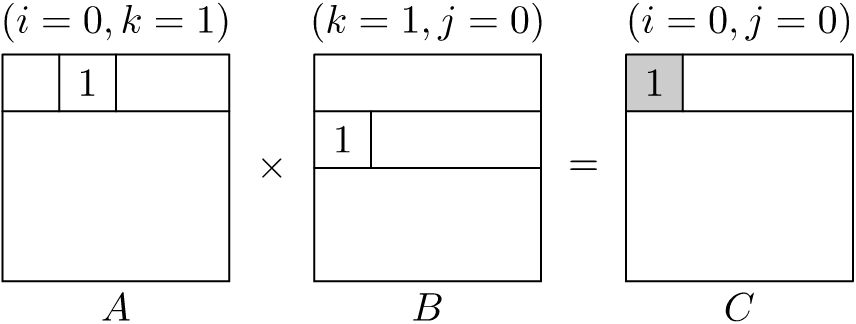
In Figure 1.5, we show the first two and last partial product-sum calculation for the innermost \(j\)-loop in matrix multiplication using the \(ikj\) loop ordering. We will be running each of these iterations for every \(ik\)-loop index combinations. If the size of the matrix is large, we can see that it is possible for the cache to be full before we reach the \(n\)th iteration. Which means that existing contents of the cache will be evicted under the cache replacement policy employed by the microprocessor (for instance, the least-recently-used (LRU) eviction policy). Hence, the values loaded in previous iterations are likely to be evicted.
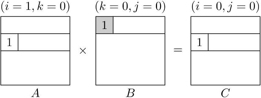
Now, if we proceed to the next iteration of the \(k\)-loop, we see the partial product-sum calculations as shown in Figure 1.6. Here, we are reusing elements of \(C\) that we had evicted in the previous innermost \(j\)-loop. This means that we are prematurely evicting and reloading the contents of \(C\) for each iteration of the \(k\)-loop. Progressing further, if we proceed to the next iteration of the outermost \(i\)-loop, we see the partial product-sum calculations as shown in Figure 1.7. Here, we are reusing elements of \(B\) that we had evicted in the previous innermost \(j\)-loop with the same \(k\)-loop index. This means that we are prematurely evicting and reloading the contents of \(B\) for each iteration of the outermost \(i\)-loop.
This means that, if we can somehow keep the prematurely evicted elements longer, we will significantly improve the performance further. Fortunately, matrix multiplication can be decomposed to partial multiplications of submatrices, an example of which is shown in \(\eqref{eqn:submatrix multiplication}\) where \(C_{i,j} = \sum_{k = 1}^3 A_{i,k}\times B_{k,j}\). Hence, if we can make at a time each of the three submatrices \(A_{i,k}\), \(B_{k,j}\) and \(C_{i,j}\) small enough that they all fit inside the cache, we will reduce premature cache evictions, thus increasing cache utilisation.
\[ \begin{align} \begin{bmatrix} A_{1,1} & A_{1,2} & A_{1,3} \\ A_{2,1} & A_{2,2} & A_{2,3} \\ A_{3,1} & A_{3,2} & A_{3,3} \end{bmatrix} \times \begin{bmatrix} B_{1,1} & B_{1,2} & B_{1,3} \\ B_{2,1} & B_{2,2} & B_{2,3} \\ B_{3,1} & B_{3,2} & B_{3,3} \end{bmatrix} = \begin{bmatrix} C_{1,1} & C_{1,2} & C_{1,3} \\ C_{2,1} & C_{2,2} & C_{2,3} \\ C_{3,1} & C_{3,2} & C_{3,3} \end{bmatrix} \label{eqn:submatrix multiplication} \end{align} \]
This takes advantage of the block multiplication method, where the entire matrix multiplication is sub-divided into block-wise multiplication of smaller submatrix blocks. By choosing the correct block size s so that all three blocks fit inside the L1 cache, we reduce the number of premature L1 cache evictions.
void matmul_ijk_block(
    float *C, const float *A, const float *B,
    size_t l, size_t m, size_t n, size_t s)
{
    <Initialise output matrix to zero>
    for (size_t ii = 0; ii < l; ii += s) {
        for (size_t jj = 0; jj < n; jj += s) {
            for (size_t kk = 0; kk < m; kk += s) {
                <Multiply block using ijk-loop order>;
            }
        }
    }
}
We multiply elements of the blocks where each block is at most s\(\times\)s large. For clarity, we calculate the elementwise pointers explicitly using their indices. In the next section, we will improve on this address calculation by replacing these multiplications with increments to elementwise pointers.
<Multiply block using ijk-loop order>=
<Check bounds and set block end indices>
for (size_t i = ii; i < ie; ++i) {
    for (size_t j = jj; j < je; ++j) {
        register float sum = 0.0;
        for (size_t k = kk; k < ke; ++k) {
            sum += *(A + i * m + k) * *(B + k * n + j);
        }
        *(C + i * n + j) += sum;
    }
}
In the outermost loops surrounding this code fragment, we increment the indices by s, which is the supplied block size. In cases where the dimensions of the original matrices are not multiples of s, we must ensure that we do not cross the matrix boundaries. Hence, we check the end of the block index against the corresponding bounds, and if it is greater, we set the block end indices to the matrix boundary. These bounds are then used inside the innermost loops.
<Check bounds and set block end indices>=
size_t ie = ii + s;
if (ie > l) {
    ie = l;
}
size_t je = jj + s;
if (je > n) {
    je = n;
}
size_t ke = kk + s;
if (ke > m) {
    ke = m;
}In this improved block multiplication, we order both the outermost block loops and the innermost block multiplication loops to follow the \(ikj\)-order. This will reduce the number of L2 and L3 cache misses, since the matrices are stored in row-major form and because of the \(ikj\)-order, the blocks will also be processed row block by row block. Note that for each row block in \(A\) and \(C\), all of the row blocks in \(B\) are processed.
void matmul_ikj_block(
    float *C, const float *A, const float *B,
    size_t l, size_t m, size_t n, size_t s)
{
    <Declare block multiplication pointers>
    <Declare and initialise row block pointers>
    <Declare block pointers>
    <Calculate size of row blocks>
    <Initialise output matrix to zero>

    for (size_t ii = 0; ii < l; ii += s) {
        B_row_block = B;
        for (size_t kk = 0; kk < m; kk += s) {
            for (size_t jj = 0; jj < n; jj += s) {
                <Multiply blocks using ikj-loop order>;
            }
            B_row_block += B_row_block_size;
        }
        A_row_block += A_row_block_size;
        C_row_block += C_row_block_size;
    }
}
These are pointers to each of the row blocks handled by the outermost loops. There will be multiple block multiplications inside each of these row blocks.
<Declare and initialise row block pointers>=
const float *A_row_block = A;
const float *B_row_block = B;
float *C_row_block = C;
Depending on the block size, we must calculate the size of each row block. This will depend on the number of columns in the original matrices.
<Calculate size of row blocks>=
size_t A_row_block_size = m * s;
size_t B_row_block_size = n * s;
size_t C_row_block_size = B_row_block_size;
These are pointers to each s\(\times\)s block inside a row block that are to be multiplied using the innermost block multiplication loops. They are initialised inside the innermost loops. During block multiplication, as we process each row in \(A\) and \(C\) blocks, we iterate through all of the rows in the \(B\) block. This is why we have an additional pointer bb which is set to the top row of the \(B\) block for each row in \(A\) and \(C\).
<Declare block pointers>=
const float *A_block;
const float *B_block;
const float *bb;
float *C_block;
These are the pointers used during block multiplication. These are the innermost loop variables which are incremented as the block elements are multiplied. Hence, they are declared as register pointers, providing a hint to the compiler.
<Declare block multiplication pointers>=
register const float *a, *b;
Inside the block multiplication loop, we first ensure that the block end indices do not cross the matrix boundaries. Then, we select the first block in each row block, and multiply these, and continue until all of the blocks in the row block is processed.
Within each block in a row block, we process the elements in \(ikj\)-order. Since the address of the elements are not explicitly calculated using indices, we simplify the innermost loops by using them as counter decrements, where each counter counts down the number of elements left to process in each dimension. Notice that the only multiplication used in the innermost loop is the multiplication required for the dot product. All elementwise addressing have been implemented using pointer increments.
In the block multiplication loop, for each element \(A_{ik}\) in the \(i\)th row and \(k\)th column in an \(A\) block, we process all of the \(j\)th column elements of the \(k\)th row in the \(B\) block and the \(i\)th row in the \(C\) block, so that the product of \(A_{ik}\) and \(B_{kj}\) is added to the current sum of products in \(C_{ij}\). Hence, for each \(k\) column element in the \(i\)th row of an \(A\) block, we update the \(i\)th row of the \(C\) block \(k\) times. Furthermore, for each \(i\)th row in the \(A\) block, all rows of the \(B\) block are used, choosing the \(k\)th row in the \(B\) block for each \(k\)th column in the \(i\)th row of the \(A\) block.
<Multiply blocks using ikj-loop order>=
<Check bounds and set block end indices>
<Set counters from block end indices>
A_block = A_row_block;
B_block = B_row_block;
C_block = C_row_block;
for (size_t i = ni; i; --i) {
    a = A_block + kk;
    bb = B_block;
    for (size_t k = nk; k; --k) {
        c = C_block + jj;
        b = bb + jj;
        <Calculate the dot product>
        bb += n;
    }
    A_block += m;
    C_block += n;
}
Since we no longer use the indices for address calculation relative to the supplied matrix pointers, we improve the loops by decrementing a counter instead.
<Set counters from block end indices>=
size_t ni = ie - ii;
size_t nj = je - jj;
size_t nk = ke - kk;
We multiply the value pointed to by a to all of the column elements pointed to by b and add these products to the corresponding existing values pointed to by c. Depending on the SIMD instructions available, we choose instructions with the highest bandwidth. If SIMD instructions are unavailable, we simply do a sequential evaluation.
<Calculate the dot product>=
#if defined(__AVX512F__)
    <Calculate the dot product with AVX-512>
#elif defined(__AVX__)
    <Calculate the dot product with AVX>
#elif defined(__SSE__)
    <Calculate the dot product with SSE>
#else
    <Calculate the dot product sequentially>
#endif
If SIMD instructions are unavailable, do a sequential evaluation by processing each element one by one.
<Calculate the dot product sequentially>=
size_t r = nj;
<Evaluate remaining elements sequentially>
The variable r stores the number of elements that remain to be evaluated, which are evaluated sequentially. This code fragment is also used by the SIMD options to evaluate elements that doesn’t fit inside a SIMD instruction.
<Evaluate remaining elements sequentially>=
if (r) {
    for (size_t j = r; j; --j) {
        *c++ += *a * *b++;
    }
}
++a;
If SSE instructions are available, we should be able to evaluate four elements in parallel with each instruction. First we divide the computation into regions that are four element multiples and evaluate these using SSE instructions, and then evaluate the remaining r elements sequentially.
<Calculate the dot product with SSE>=
size_t r = nj % 4;
__m128 a_ = _mm_set1_ps(*a);
for (size_t j = nj - r; j; j -= 4) {
    __m128 b_ = _mm_loadu_ps(b);
    __m128 c_ = _mm_loadu_ps(c);
    b_ = _mm_mul_ps(a_, b_);
    c_ = _mm_add_ps(c_, b_);
    _mm_storeu_ps(c, c_);
    b += 4;
    c += 4;
}
<Evaluate remaining elements sequentially>
If AVX instructions are available, we should be able to evaluate eight elements in parallel with each instruction. Similar to the SSE method, first we divide the computation into regions that are eight element multiples and evaluate these using AVX instructions, and then evaluate the remaining r elements sequentially.
<Calculate the dot product with AVX>=
size_t r = nj % 8;
__m256 a_ = _mm256_set1_ps(*a);
for (size_t j = nj - r; j; j -= 8) {
    __m256 b_ = _mm256_loadu_ps(b);
    __m256 c_ = _mm256_loadu_ps(c);
    b_ = _mm256_mul_ps(a_, b_);
    c_ = _mm256_add_ps(c_, b_);
    _mm256_storeu_ps(c, c_);
    b += 8;
    c += 8;
}
<Evaluate remaining elements sequentially>
If AVX-512 instructions are available, we should be able to evaluate sixteen elements in parallel with each instruction. The rest is similar to the AVX option.
<Calculate the dot product with AVX-512>=
size_t r = nj % 16;
__m512 a_ = _mm512_set1_ps(*a);
for (size_t j = nj - r; j; j -= 16) {
    __m512 b_ = _mm512_loadu_ps(b);
    __m512 c_ = _mm512_loadu_ps(c);
    b_ = _mm512_mul_ps(a_, b_);
    c_ = _mm512_add_ps(c_, b_);
    _mm512_storeu_ps(c, c_);
    b += 16;
    c += 16;
}
<Evaluate remaining elements sequentially>We now implement \(AB^T\) and \(A^TB\), but without first doing a transpose. Let’s start with \(AB^T\), as it is simpler.
The memory access pattern for \(AB^T\) using the \(ijk\)-loop ordering, where we use the transposed matrix \(B^T\) is as follows:

If we look at the memory access pattern of \(AB^T\) with the same loop ordering, but using the matrix \(B\) before it was transposed, we see:
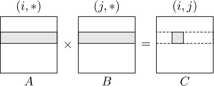
This shows that the cache utilisation is optimal since all memory accesses utilise all values in the cache (although cache evictions still occur with same cache lines reloaded again). The elements of each row in both the input matrix and the output matrix are accessed and updated sequentially when using the \(ijk\)-loop ordering.
The matrix multiplication \(AB^T\) can therefore be implemented simply as follows, where \(B\) is the matrix before transposition:
void abT_matmul_ijk(
    float *C, const float *A, const float *B,
    size_t l, size_t m, size_t n)
{
    <<Initialise output matrix to zero>>
    for (size_t i = 0; i < l; ++i) {
        register const float *b = B;
        for (size_t j = 0; j < n; ++j) {
            register const float *a = A;
            register float s = 0.0;
            for (size_t k = 0; k < m; ++k) {
                s += *a++ * *b++;
            }
            *C++ = s;
        }
        A += m;
    }
}
For every row of \(A\), we iterate through every row of \(B\). Every dot product between a row of \(A\) with a row of \(B\) produces an element in \(C\). When we visit every row of \(B\) against a row of \(A\), the resulting dot products are sequential elements in \(C\). Hence, we can continue to calculate every element of \(C\) sequentially starting at the first location, and ending at the last element.
For \(A\) as well, we start at the first element of the first row and process every element of that row sequentially. We do the same for all of the remaining rows. Notice, however, that for every row in \(B\), we must start at the first element of the current row in \(A\), hence, the resetting of a inside the \(j\)th loop. Of course, once the \(j\) loop has completed, we move to the next row of \(A\) by jumping by \(m\) elements. These resetting of a to the beginning of each row may require reloading elements to the cache.
For the \(B\) matrix, all elements are accessed sequentially for each row in \(A\), hence, we reset b to the first element of \(B\) inside the \(i\)th loop. This will also require reloading elements of \(B\) to the cache. We do not update the elements of \(C\) once it has been calculated, as the dot product is not split into multiple phases. This is carried out using the variable s.
Implementation of \(A^TB\) is slightly more complicated. If we look at the memory access pattern for \(A^TB\) using the \(ijk\)-loop ordering, where \(A^T\) is the already transposed matrix, we observe the following pattern:
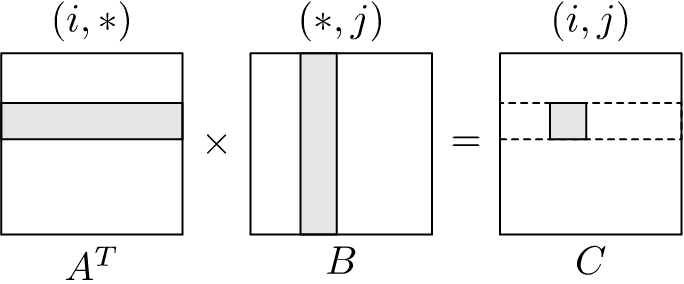
If we look at the memory access pattern of \(A^TB\) with the same loop ordering, but using the matrix \(A\) before it was transposed, we see:
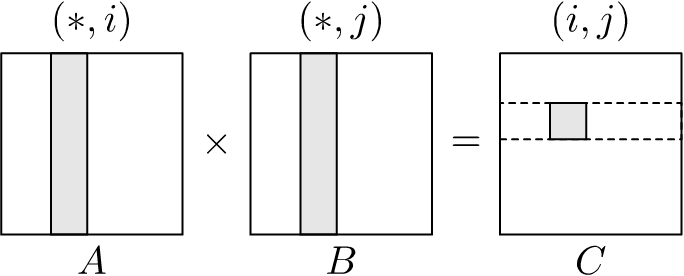
This means that we must not produce the required dot products in a single loop, as was the case with \(AB^T\), but split it into multiple phases. This will allow us to access all of the required elements in \(A\), \(B\) and \(C\) sequentially. We implement this as follows, where \(A\) is the matrix before transposition:
void aTb_matmul_kij(
    float *C, const float *A, const float *B,
    size_t l, size_t m, size_t n)
{
    register const float *a = A;
    <<Initialise output matrix to zero>>
    for (size_t k = 0; k < m; ++k) {
        c = C;
        for (size_t i = 0; i < l; ++i) {
            register const float *b = B;
            for (size_t j = 0; j < n; ++j) {
                *c++ += *a * *b++;
            }
            ++a;
        }
        B += n;
    }
}
From the memory access pattern shown in Figure 1.11, we first notice that for every column of \(A\) we iterate against all columns of \(B\) starting with the first column of \(B\) accessing all columns sequentially. Furthermore, every row of \(A\) results in a row of \(C\), and every column of \(B\) results in a column in \(C\). This means that we can start at the first element of \(C\) and update each of the elements sequentially with partial dot products until it has updated its final element. Then, it rewinds back to the first element of \(C\), and continue the process until the dot products are complete. Hence, we loop through all elements of \(C\) sequentially \(m\) times, manifested in the outermost \(k\) loop. These will require cache reload of elements in \(C\).
The memory access pattern for \(A\) is slightly simpler as it does not require rewinding. We start at the first row of \(A\) and continue processing all of its elements sequentially. Of course, we use the same element of \(A\) while calculating each of the \(n\) partial dot products with a row of \(B\), which we do inside the innermost \(j\) loop. Once a row of \(B\) has been processed, we then move to the next sequential element of \(A\).
The memory access pattern for \(B\) requires rewinding for every new row of \(A\), so that for every element of \(A\) in a row, we process all elements of a row in \(B\), rewinding at the beginning of the row for each row element in \(A\). Hence, \(B\) will require cache reloads. This is done in the \(i\)th loop. Of course, once a row of \(A\) has been processed, we jump to the next row of \(B\). Again, all elements of \(B\) are accessed sequentially improving cache utilisation.
Since the elements of \(C\) are calculated using multiple partial dot products, we must initialise the result matrix \(C\) to zero prior to entering the outermost loop.
We plan to include bench-marking information of the variants discussed in this article. At the moment we have not figured out how to use block multiplication to improve on the cache reloads in in-place multiplications involving transposition. Furthermore, we are yet to implement \(A^TB\) and \(AB^T\) using SIMD intrinsics.
While writing this article, we found the following materials helpful:
Recent developments in improving the performance of matrix multiplication using artificial intelligence (AlphaTensor) is interesting. This is related to the block multiplication we discussed previously, and how the Strassen algorithm allows us to reduce the number of block multiplications (while increasing the number of additions) required to produce the final matrix multiplication. We plan to discuss this further in a separate article.
