16 December 2020, Wednesday
The key to understanding convolution is to imagine real life situations where it is applicable. Two such examples concern echoes and blurring. They provide two imaginable contexts that helped me understand both the temporal and spatial aspects of a convolution. The echoes example enlightens the temporal perspective of convolution, whereas optical blurring provides a spatial interpretation.
When studying convolution, we always arrive at one important question: how is convolution different from cross-correlation? In fact, this was the part which I struggled with the most; but once the difference was clear, convolution felt intuitive. It even brought out the convolution equation naturally. To understand this better, let us start with cross-correlation.
Let’s say we have two integer-valued row vectors \(A\) and \(B\) such that \(A = \begin{bmatrix}1 & 2 & 3\end{bmatrix}\) and \(B = \begin{bmatrix}4 & 5 & 6\end{bmatrix}\). The cross-correlation of these two vectors is:
\[A \star B = \begin{bmatrix}6 & 17 & 32 & 23 & 12\end{bmatrix}.\]
Note that cross-correlation is denoted by the \(\star\) symbol. How is this cross-correlation calculated? As shown below, cross-correlation is calculated by shifting one of the vectors relative to the other, then multiplying aligned pairs that are finally added together. We do this for all possible shifts that result in an overlap between the vectors.
\[ \begin{align*} & 1\, 2\, 3\\ 4\, 5\, & 6\\ & 1 \times 6 \rightarrow 6 \end{align*} \]
\[ \begin{align*} & 1\, 2\, 3\\ 4\, & 5\, 6\\ & 1 \times 5 + 2 \times 6 \rightarrow 17 \end{align*} \]
\[ \begin{align*} & 1\, 2\, 3\\ & 4\, 5\, 6\\ & 1 \times 4 + 2 \times 5 + 3 \times 6 \rightarrow 32 \end{align*} \]
\[ \begin{align*} 1\, & 2\, 3\\ & 4\, 5\, 6\\ & 2 \times 4 + 3 \times 5 \rightarrow 23 \end{align*} \]
\[ \begin{align*} 1\, 2\, & 3\\ & 4\, 5\, 6\\ & 3 \times 4 \rightarrow 12 \end{align*} \]
Now, if we look at the convolution of these same two vectors, which is denoted by the \(*\) symbol, we get a different result:
\[A * B = \begin{bmatrix}4 & 13 & 28 & 27 & 18\end{bmatrix}.\]
The convolution is calculated as follows:
\[ \begin{align*} & 1\, 2\, 3\\ 6\, 5\, & 4\\ & 1 \times 4 \rightarrow 4 \end{align*} \]
\[ \begin{align*} & 1\, 2\, 3\\ 6\, & 5\, 4\\ & 1 \times 5 + 2 \times 4 \rightarrow 13 \end{align*} \]
\[ \begin{align*} & 1\, 2\, 3\\ & 6\, 5\, 4\\ & 1 \times 6 + 2 \times 5 + 3 \times 4 \rightarrow 28 \end{align*} \]
\[ \begin{align*} 1\, & 2\, 3\\ & 6\, 5\, 4\\ & 2 \times 6 + 3 \times 5 \rightarrow 27 \end{align*} \]
\[ \begin{align*} 1\, 2\, & 3\\ & 6\, 5\, 4\\ & 3 \times 6 \rightarrow 18 \end{align*} \]
They both seem to be doing the same thing, except, in a convolution, we flip one of the vectors. The question is, why? This flipping operation confused me the most. Various explanations of convolution simply gloss over this fundamental operation by providing the convolution formula, with little explanation on why it is necessary to flip one of the vectors. In fact, for a two dimensional convolution, we must flip one of the matrices being convolved both vertically and horizontally.
In the following sections, I discuss two ways of understanding this. Let’s begin with optical blurring, which does not have special cases to consider. This will be followed by the case for echoes, which does have a special case to consider, because of the fact that time cannot flow backward. While reading the following, always remember that we are working with two frames of reference, each fixed to one of the objects that we are convolving.
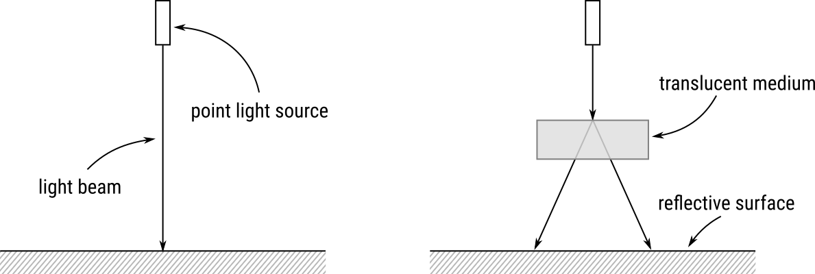
Imagine you have a point source of light that falls on a piece of translucent plastic. The plastic will scatter the beam of light, and when the light falls on a reflective surface, we get a blurry spot of light instead of a sharp point of light. The following diagram illustrates this:
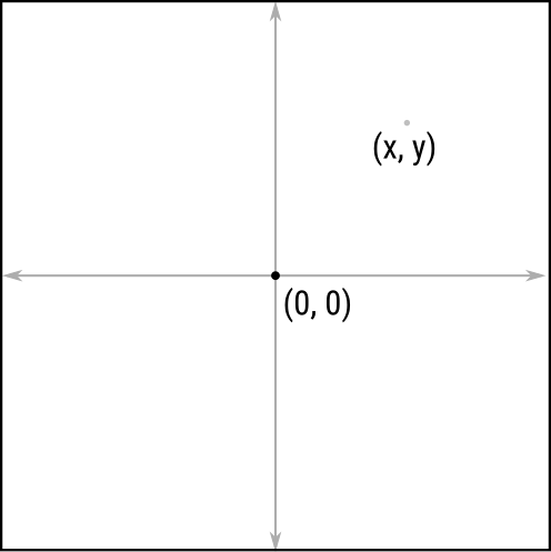
If we imagine looking from the above, we will see something similar to the following:

Now, imagine that each of the points on the reflecting surface is given a coordinate \((x, y)\), and that the center of the light beam coincides with the origin of this coordinate system, as shown below:
We can then ask how we would define blurring when we introduce the translucent plastic in the path of the light beam. In the case when there is no blurring, we have the intensity of light, say \(I\), at the origin \((0, 0)\); and zero intensity for all of the other points. On the other hand, when we have blurring, the intensity at the origin \((0, 0)\) is a fraction of \(I\), since some of that light have been scattered to nearby points. This means that few of the nearby points that used to have zero intensity will now have a fraction of the intensity \(I\), the amount determined by the properties of the translucent plastic. A function that provides the intensity for a given point on the reflecting surface is referred to as a point spread function. Hence, different mediums will have different point spread functions.
Once we run this function over a region of the reflecting surface, we get a matrix of intensity values as shown below. This is referred to as the convolution kernel. Why? Because, if we had an array of point sources of light instead of just one single point source, we can calculate the intensity on the reflecting surface by convolving the point source intensity matrix with the convolution kernel that corresponds to the point spread function of the blurring medium. This will become clearer once we consider an example.
Let us quantize the reflecting surface into a rectangular grid of squares as follows:
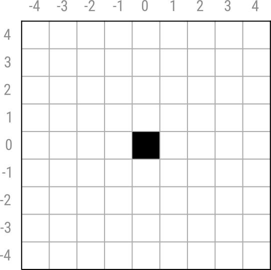
Assume that the point light falls at the center of this grid, which is the square with coordinates \((5, 5)\). When there is no blurring we will have the convolution kernel specified by the discrete point spread function \(f\), defined as follows:
\[ f(x,y,I) = \begin{cases} I & \textrm{if } x = 5\textrm{ and } y = 5\textrm{, and}\\ 0 & \textrm{otherwise.} \end{cases} \]
Now, if we introduce a blurring medium that has a gaussian point spread function, \(f'\), then we will have:
\[ f'(x,y,I) = I \exp\left[- \left(\frac{(x-x_o)^2}{2\sigma_X^2} + \frac{(y-y_o)^2}{2\sigma_Y^2} \right)\right]. \]
Here, \((x_o, y_o)\) is the origin, which in our case is \(x_o = 5\) and \(y_o = 5\). The variables \(\sigma_X\) and \(\sigma_Y\) respectively give the standard deviations of the gaussian distribution in the \(x\) and \(y\) directions. Now, don’t worry too much about the above function. What really matters is that for all squares on the grid, we will get an intensity fraction dictated by the point spread function of the medium. Hence, if we used a standard gaussian with unit standard deviations (i.e., \(\sigma_X = \sigma_Y = 1\)) and assume unit intensity, \(I = 1\), we get a convolution kernel \(k\) similar to the following (with a visual using inverted colour to the right):
| 0.000 | 0.000 | 0.000 | 0.000 | 0.000 | 0.000 | 0.000 | 0.000 | 0.000 |
| 0.000 | 0.000 | 0.002 | 0.007 | 0.011 | 0.007 | 0.002 | 0.000 | 0.000 |
| 0.000 | 0.002 | 0.018 | 0.082 | 0.135 | 0.082 | 0.018 | 0.002 | 0.000 |
| 0.000 | 0.007 | 0.082 | 0.368 | 0.607 | 0.368 | 0.082 | 0.007 | 0.000 |
| 0.000 | 0.011 | 0.135 | 0.607 | 1.000 | 0.607 | 0.135 | 0.011 | 0.000 |
| 0.000 | 0.007 | 0.082 | 0.368 | 0.607 | 0.368 | 0.082 | 0.007 | 0.000 |
| 0.000 | 0.002 | 0.018 | 0.082 | 0.135 | 0.082 | 0.018 | 0.002 | 0.000 |
| 0.000 | 0.000 | 0.002 | 0.007 | 0.011 | 0.007 | 0.002 | 0.000 | 0.000 |
| 0.000 | 0.000 | 0.000 | 0.000 | 0.000 | 0.000 | 0.000 | 0.000 | 0.000 |

What this kernel is really saying is that if we have a beam of light at the origin \((5, 5)\) with an intensity of 1 unit, which then passes through a medium with standard gaussian point spread function, the intensity at the origin is 1 (say, the medium does not introduce a loss); squares adjacent to this origin vertically and horizontally will have intensities 0.607, whereas, squares adjacent diagonally to the origin will have intensity 0.368. As we get farther from the origin, the intensity decreases.
The next question is, what if the beam of light is not incident at the origin, but is incident on some other square on the grid, say \((3, 3)\). In that case, we will see a blurred spot of light that has been shifted, as shown below:
| 0 | 0 | 0 | 0 | 0 | 0 | 0 | 0 | 0 |
| 0 | 0 | 0 | 0 | 0 | 0 | 0 | 0 | 0 |
| 0 | 0 | 1 | 0 | 0 | 0 | 0 | 0 | 0 |
| 0 | 0 | 0 | 0 | 0 | 0 | 0 | 0 | 0 |
| 0 | 0 | 0 | 0 | 0 | 0 | 0 | 0 | 0 |
| 0 | 0 | 0 | 0 | 0 | 0 | 0 | 0 | 0 |
| 0 | 0 | 0 | 0 | 0 | 0 | 0 | 0 | 0 |
| 0 | 0 | 0 | 0 | 0 | 0 | 0 | 0 | 0 |
| 0 | 0 | 0 | 0 | 0 | 0 | 0 | 0 | 0 |
| 0.018 | 0.082 | 0.135 | 0.082 | 0.018 | 0.002 | 0.000 | 0.000 | 0.000 |
| 0.082 | 0.368 | 0.607 | 0.368 | 0.082 | 0.007 | 0.000 | 0.000 | 0.000 |
| 0.135 | 0.607 | 1.000 | 0.607 | 0.135 | 0.011 | 0.000 | 0.000 | 0.000 |
| 0.082 | 0.368 | 0.607 | 0.368 | 0.082 | 0.007 | 0.000 | 0.000 | 0.000 |
| 0.018 | 0.082 | 0.135 | 0.082 | 0.018 | 0.002 | 0.000 | 0.000 | 0.000 |
| 0.002 | 0.007 | 0.011 | 0.007 | 0.002 | 0.000 | 0.000 | 0.000 | 0.000 |
| 0.000 | 0.000 | 0.000 | 0.000 | 0.000 | 0.000 | 0.000 | 0.000 | 0.000 |
| 0.000 | 0.000 | 0.000 | 0.000 | 0.000 | 0.000 | 0.000 | 0.000 | 0.000 |
| 0.000 | 0.000 | 0.000 | 0.000 | 0.000 | 0.000 | 0.000 | 0.000 | 0.000 |
What if the beam was still incident at \((3, 3)\) but now has an intensity of 2 units? Assuming that the properties of the medium does not depend on the intensity of the incident light, we can simply multiply the convolution kernel with a scaling factor of \(2\), to give the following blurred spot on the reflecting surface.
| 0 | 0 | 0 | 0 | 0 | 0 | 0 | 0 | 0 |
| 0 | 0 | 0 | 0 | 0 | 0 | 0 | 0 | 0 |
| 0 | 0 | 2 | 0 | 0 | 0 | 0 | 0 | 0 |
| 0 | 0 | 0 | 0 | 0 | 0 | 0 | 0 | 0 |
| 0 | 0 | 0 | 0 | 0 | 0 | 0 | 0 | 0 |
| 0 | 0 | 0 | 0 | 0 | 0 | 0 | 0 | 0 |
| 0 | 0 | 0 | 0 | 0 | 0 | 0 | 0 | 0 |
| 0 | 0 | 0 | 0 | 0 | 0 | 0 | 0 | 0 |
| 0 | 0 | 0 | 0 | 0 | 0 | 0 | 0 | 0 |
| 0.037 | 0.164 | 0.271 | 0.164 | 0.037 | 0.003 | 0.000 | 0.000 | 0.000 |
| 0.164 | 0.736 | 1.213 | 0.736 | 0.164 | 0.013 | 0.000 | 0.000 | 0.000 |
| 0.271 | 1.213 | 2.000 | 1.213 | 0.271 | 0.022 | 0.001 | 0.000 | 0.000 |
| 0.164 | 0.736 | 1.213 | 0.736 | 0.164 | 0.013 | 0.000 | 0.000 | 0.000 |
| 0.037 | 0.164 | 0.271 | 0.164 | 0.037 | 0.003 | 0.000 | 0.000 | 0.000 |
| 0.003 | 0.013 | 0.022 | 0.013 | 0.003 | 0.000 | 0.000 | 0.000 | 0.000 |
| 0.000 | 0.000 | 0.001 | 0.000 | 0.000 | 0.000 | 0.000 | 0.000 | 0.000 |
| 0.000 | 0.000 | 0.000 | 0.000 | 0.000 | 0.000 | 0.000 | 0.000 | 0.000 |
| 0.000 | 0.000 | 0.000 | 0.000 | 0.000 | 0.000 | 0.000 | 0.000 | 0.000 |
Hence, in general, if we have a light source of intensity \(I\), we simply multiply the convolution kernel with that intensity. But for this to be feasible, the convolution kernel must be expressed in relation to a unit signal intensity by setting \(I = 1\) in \(f'(x,y,I)\) above. This is referred to as the unit impulse response, since the beam of light is conceptually treated as a discrete impulse on the two dimensional grid, which then produced the blurred response on the reflecting surface.
We are now ready to understand convolution, and it hinges on one question: What if we have two point sources of light each incident at \((3, 3)\) and \((5, 5)\) with respective intensities 3 and 1? How would the blurred light appear on the reflective surface? The following (on the right) is what you will get, and this is the result of convolving the standard gaussian unit impulse response \(k\), defined above, with the signal, which is the matrix on the left.
| 0 | 0 | 0 | 0 | 0 | 0 | 0 | 0 | 0 |
| 0 | 0 | 0 | 0 | 0 | 0 | 0 | 0 | 0 |
| 0 | 0 | 2 | 0 | 0 | 0 | 0 | 0 | 0 |
| 0 | 0 | 0 | 0 | 0 | 0 | 0 | 0 | 0 |
| 0 | 0 | 0 | 0 | 1 | 0 | 0 | 0 | 0 |
| 0 | 0 | 0 | 0 | 0 | 0 | 0 | 0 | 0 |
| 0 | 0 | 0 | 0 | 0 | 0 | 0 | 0 | 0 |
| 0 | 0 | 0 | 0 | 0 | 0 | 0 | 0 | 0 |
| 0 | 0 | 0 | 0 | 0 | 0 | 0 | 0 | 0 |
| 0.037 | 0.164 | 0.271 | 0.164 | 0.037 | 0.003 | 0.000 | 0.000 | 0.000 |
| 0.164 | 0.736 | 1.215 | 0.742 | 0.175 | 0.020 | 0.002 | 0.000 | 0.000 |
| 0.271 | 1.215 | 2.018 | 1.295 | 0.406 | 0.104 | 0.019 | 0.002 | 0.000 |
| 0.164 | 0.742 | 1.295 | 1.104 | 0.771 | 0.381 | 0.082 | 0.007 | 0.000 |
| 0.037 | 0.175 | 0.406 | 0.771 | 1.037 | 0.610 | 0.135 | 0.011 | 0.000 |
| 0.003 | 0.020 | 0.104 | 0.381 | 0.610 | 0.368 | 0.082 | 0.007 | 0.000 |
| 0.000 | 0.002 | 0.019 | 0.082 | 0.135 | 0.082 | 0.018 | 0.002 | 0.000 |
| 0.000 | 0.000 | 0.002 | 0.007 | 0.011 | 0.007 | 0.002 | 0.000 | 0.000 |
| 0.000 | 0.000 | 0.000 | 0.000 | 0.000 | 0.000 | 0.000 | 0.000 | 0.000 |
Visually, the blurred light will appear in inverted colour as shown below:

From this, we can see that the blurred response for the two point sources is the sum of the individual impulse response multiplied by their intensities. For instance, the intensity at square \((5, 5)\) is the sum of the impulse response for source with intensity 1 at \((5, 5)\), which is 1; and the impulse response for the source with intensity 2 at \((3, 3)\), which is 0.037, thus giving the resultant intensity 1.037. We can determine the resultant intensities for the rest of the squares in the grid.
Of course, in this example, because the convolution kernel is symmetric, we won’t see why convolution requires flipping the kernel. So, to assist with that, and to bring out the fundamental idea, let us use two smaller matrices representing signal, \(S\) and kernel, \(K\), and ensure that the kernel is not symmetric. The following example matrices will do:
\[ S = \begin{bmatrix} 1 & 2 & 3\\ 4 & 5 & 6\\ 7 & 8 & 9 \end{bmatrix} \]
\[ K = \begin{bmatrix} 10 & 11 & 12\\ 13 & 14 & 15\\ 16 & 17 & 18 \end{bmatrix} \]
\[ S*K = \begin{bmatrix} 134 & 245 & 198\\ 327 & 570 & 441\\ 350 & 587 & 438 \end{bmatrix} \]
What the signal matrix \(S\) is saying is that we now have nine point sources of light, each with intensities from 1 to 9 ordered in row-major form on the \(3\times 3\) point source grid. So, if we wanted to find the resultant intensity on a square at grid position, say \((2, 2)\), which the convolution has shown to have a value of 570, how would we calculate this? It’s simple. We simply add the contributions from all of the nine point sources to square \((2, 2)\). Hence, if we consider the point source at \((1, 1)\) with intensity 1, what would be its contribution to point \((2, 2)\)? We look at the convolution kernel and first place the origin of the kernel on top of the point source. We then determine the value of the kernel at point \((2, 2)\) on the grid coordinate system, which is equivalent to point \((3, 3)\) on the kernel coordinate system. The value is 18. So, the contribution of intensity 1 at \((1, 1)\) to point \((2, 2)\) is \(1\times 18\). Similarly, the contribution of intensity 2 point at \((1, 2)\) is \(2 \times 17\), and so on, thus giving us the final value:
\[ 570 = 1\times 18 + 2\times 17 + 3\times 16 + 4\times 15 + 5\times 14 + 6\times 13 + 7\times 12 + 8\times 11 + 9\times 10 \]
In general, if we wish to calculate the resultant value at point \((u, v)\) on the surface grid, we must add the contributions from all point sources on the signal grid, \((x, y)\) where \(x = 1,\ldots,3\) and \(y = 1,\ldots,3\). The contribution of a point source at \((x, y)\) is given by the product of the intensity at \((x, y)\), which is \(S(x, y)\), and the point spread due to the blurring effect of the convolution kernel, which is given by \(K(x', y')\) where \((x', y')\) is the kernel coordinate that corresponds to the point source coordinate \((u, v)\) on the surface grid coordinate system. If we do the translation, we get \(x' = x - u\) and \(y' = y - v\). In fact, this is what causes the flipping of the kernel! This translation is shown visually in the following diagram.

Thus, we can write discrete convolution as follows:
\[[S * K]_{u,v} = \sum_{\substack{1 \le x \le 3\\1 \le y \le 3}}S(x,y) . K(u - x, v - y)\]
By \([S * K]_{u,v}\), we mean value of the \(S*K\) matrix at row \(u\) and column \(v\). Note that when \(u - x < 1\) or \(u - x > 3\), or \(v - y < 1\) or \(v - y > 3\), we assume that the value of \(K(u - x, v - y)\) equals zero. This is a reasonable assumption since we can imagine that the kernel is an infinite grid with default zero values. Furthermore, we can also assume that the signal grid extends to infinity, and that the squares in both grids are infinitesimally small. Under these assumptions, we can define both the signal and the convolution kernels as continuous functions \(s(x,y)\) and \(k(x',y')\) respectively, such that the value of the continuous convolution at a point \((u, v)\) is given by:
\[(s*k)(u,v) = \int_{-\infty}^{\infty}\int_{-\infty}^{\infty}s(x,y).k(u-x,v-y) \,dx \,dy\]
This shown that in a spatial sense, a convolution calculates the resultant effects of point spread contributions from all points of a signal, where the contribution for each signal point to its neighbouring points is calculated using a point spread function, which is the convolution kernel. In the next section, we discuss the temporal interpretation which is very similar to the spatial interpretation, except that the resultant effect in the future is calculated by summing contributions from signal points in the past.
Imagine that you are inside a silent cave in the mountains, and that you clap once. Depending on the loudness of your clap and the character of the cave—for instance, the orientation of the cave surfaces and the sound properties of the rock—you will hear echoes of the clap. This is shown in the diagram below.
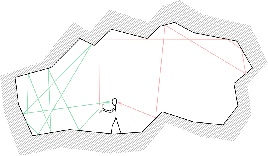
Depending on the direction of the sound waves produced by your clap, these waves will travel for different durations bouncing from surface to surface until it reaches your ears. Hence, as you listen quietly, the intensity of the sound you hear will change as a function of time, where at each time point the sound intensity you hear is the resultant intensity of the sound waves reaching your ears at that time point. This is shown in the following plot.
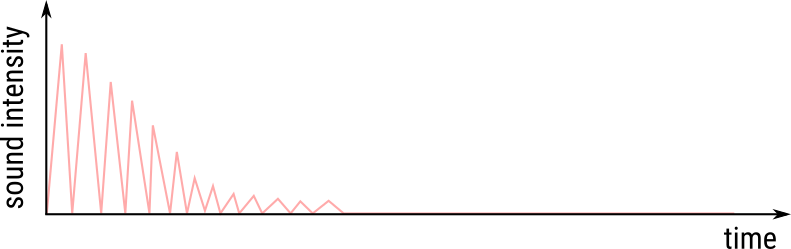
What this really means is that the effect of the clapping event persist through time thus generating the sound your ears hear even after you have finished clapping. Now, if the surface of the cave does not reflect sound then you will not hear any echoes, as the sound waves which left the clapping hands will not return. Of course, you will still hear the initial sound waves that went straight from the hands to the ears. But you will not hear any echoes.
Hence, the existence of sound reflecting surfaces is similar to the introduction of a blurring medium that we discussed in the previous section. However, instead of affecting the spatial neighbourhood which was the case with blurring, the existence of the reflecting cave surface affects the temporal neighbourhood. Since time flows forward, the clapping event cannot affect the past; it can only affect the future. This is the special case we mentioned at the beginning of this article. With blurring the spatial effect is not limited, whereas, with clapping, the effect can only persist in the future and not affect the past. Thus, for the clap event, we can define a function \(g(t)\) that gives the sound intensity heard through time \(t\) for a clap of intensity 1 unit. Since time flows forward, \(t \ge 0\), with \(t=0\) marking the event when the clapping finished. This function is similar to the point spread function, of course with the special case where \(g(t) = 0\) when \(t < 0\). This is the convolution kernel for the clapping inside this cave at the position where you stand.
Now, imagine that you clap two times at the same spot inside the same cave instead of clapping just once. The first clap happens at time \(t=0\), which is followed by the second clap at time \(t=\tau\). Given that both claps have the same convolution kernel \(g(t)\), what would you hear through time? In other words, if we represent with \(s(t)\) the sound intensity that you hear at time \(t\), what would you hear at some future time \(t=\kappa\) after the second clap? The answer is again given by convolution. If we define the convolution kernel as a unit impluse response function, then we can even ask what \(s(t)\) will be at time \(t=\kappa\) after the second clap, where the first clap had an intensity two units while the second clap had an intensity of four units?
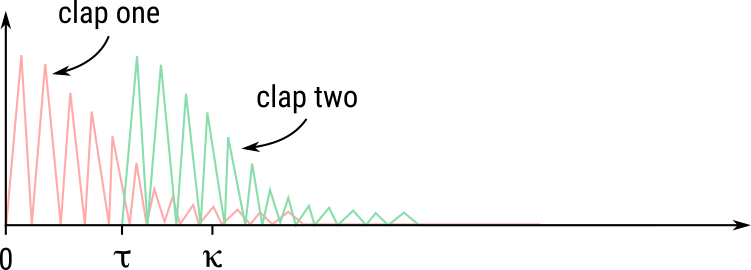
Just as before, we can evaluate this by considering contribution of each compoent separately at time \(t=\kappa\). For the first clap, the contribution time \(t=\kappa\) is given by the value of the convolution kernel, which is \(g(\kappa)\). For the second clap, the contribution at time \(t=\kappa\) will be given by \(g(\kappa - \tau)\) because, at time \(t=\kappa\), the time for the sound waves generated by the second clap at time \(t=\tau\) has only elapsed for \((\kappa - \tau)\) time uints. Thus, when looking up the contribution for the second clap, we must choose the value at time point \((\kappa - \tau)\). Hence, if the first clap has intensity \(a\) and second clap had intensity \(b\), we can the resultant sound intensity at time \(t = \kappa\) as \(a \times g(\kappa) + b \times g(\kappa - \tau)\).
Now, imagine that we clap at every time point following the first clap and that the intensity of each clap is given by the function \(f(t)\), then the resultant sound intensity heard at time \(t=\kappa\) will be given by
\[(f*g)(\kappa) = \int_{0}^{\tau}f(\tau).g(\kappa - \tau) \,d\tau.\]
For the discrete case, we have
\[(F * G)[i] = \sum_{j=0}^{N}F[j].G[i - j]\]
where, \((F*G)[i]\) denotes the \(i\)th element (assuming indexing begins at 0) of the \(F*G\) convolution vector; similarly, for \(F\) and \(G\) vectors. The constant \(N\) gives the number of elements in \(F\). As before, value of \(G[i]\) is assumed zero if the index \(i\) is outside the valid range determined by the size of the convolution kernel \(G\).
For our example, which produced the convolution \(A * B = \begin{bmatrix}4 & 13 & 28 & 27 & 18\end{bmatrix}\), we can see the indexing as follows:
| j | i=0 | i=1 | i=2 | i=3 | i=4 |
| 0 | A[0]=1, B[ 0]=4 | A[0]=1, B[ 1]=5 | A[0]=1, B[ 2]=6 | A[0]=1, B[3]=0 | A[0]=1, B[4]=0 |
| 1 | A[1]=2, B[-1]=0 | A[1]=2, B[ 0]=4 | A[1]=2, B[ 1]=5 | A[1]=2, B[2]=6 | A[1]=2, B[3]=0 |
| 2 | A[2]=3, B[-2]=0 | A[2]=3, B[-1]=0 | A[2]=3, B[ 0]=4 | A[2]=3, B[1]=5 | A[2]=3, B[2]=6 |
| 3 | A[3]=0, B[-3]=0 | A[3]=0, B[-2]=0 | A[3]=0, B[-1]=0 | A[3]=0, B[0]=4 | A[3]=0, B[1]=5 |
| 4 | 13 | 28 | 27 | 18 |
In general, the continuous one-dimensional convolution is a function of \(t\), where
\[(f*g)(t) = \int_{-\infty}^{\infty}f(\tau).g(t - \tau) \,d\tau.\]
When returning the convolution of two matrices or vectors, there are two ways of returning the values. In the first case, we return the full convolution, as with the vector convolution above. The number of elements in the convolution equals \(|A|+|B|-1\), where \(|A|\) denotes the number of elements in \(A\); similarly for \(B\). On the other hand, we can return only the middle portion of the convolution so that the dimension of the returned matrix or vector matches the dimension of the signal matrix. This case is covered by convolution \(S*K\) for the blurring example above. If, on the other hand, we chose to return the full convolution for \(S*K\), we will get:
\[ S*K = \begin{bmatrix} 10 & 31 & 64 & 57 & 36\\ 53 & 134 & 245 & 198 & 117\\ 138 & 327 & 570 & 441 & 252\\ 155 & 350 & 587 & 438 & 243\\ 112 & 247 & 406 & 297 & 162 \end{bmatrix} \]
I read the article on convolution by BetterExplained a few weeks a ago. Although the article is excellent, there were a few things which I was not clear about. This is my attempt to fill in that gap in my understanding. I have been working with convolutions for a while in relation to image processing, but my intuitive understanding was always wanting. Finally, after thinking about it a bit more following the mentioned article, I think I finally understand it. Of course, several stack overflow articles provided hints and clues from various perspectives which helped my understand.
