30 May 2024, Thursday
Statistical analysis of performance improvements due to optimisation techniques
How do you measure and compare application performance, and how to be sure any performance improve due to certain optimisation techniques is not a fluke? How do you compare and choose between optimisation strategies?
This is a digression from my notes on my GPT-2 experiments; however, I felt that it was necessary for me to understand, and articulate, how to measure performance improvements due to changes in optimisation strategies, and how to be sure the changes are indeed causing the observed improvements.
We measure systematically, and then explain statistically, accounting for random fluctuations.
Of course, it may be extremely difficult to do this for a more complex optimisation scenario, however, I felt that the example problem of token embedding and positional encoding is simple enough that we can appreciate the value of possible optimisations. In fact, a lot of the processing inside the GPT-2 architecture seems to be variations on this processing pattern. The other pattern is reduction, which we shall investigate when we address layer normalisation.
We use our SIMD parallelisation of the GPT-2 token embedding and positional encoding application (see GPT-2 parallelisation: embedding with SIMD (part 1)). The code was written in a form that allows for selection of parallelisation strategies using compiler flags.
We generate multiple binaries by enabling and disabling compile flags
that affect the instructions used. These are summarised as follows (see
Generating the binaries below for
the corresponding Makefile configs):
| SSE | AVX | OMP | Pointer | |
|---|---|---|---|---|
| embed_seq | ✗ | ✗ | ✗ | - |
| embed_avx | ✓ | ✓ | ✗ | - |
| embed_sse | ✓ | ✗ | ✗ | - |
| embed_normal | - | - | - | - |
| embed_seq_omp | ✗ | ✗ | ✓ | - |
| embed_sse_omp | ✓ | ✗ | ✓ | - |
| embed_avx_omp_ptr | ✓ | ✓ | ✓ | ✓ |
| embed_avx_omp | ✓ | ✓ | ✓ | ✗ |
Note here that we implemented the AVX version with OpenMP multi-threading using both pointer arithmetic and counter method (how we maintain the number of items processed respectively by the AVX, SSE and scalar instructions). This does not apply to the remaining optimisations.
The next question is, how many times should we run each binary file to account for statistical variations? It is important to note that since we will be comparing between multiple strategies (i.e., multiple binaries) we have to take into account the statistical power for discriminating between the performances of the binaries, how big a difference we expect to discern (the effect size), and how sure we want to be (the statistical significance threshold). These are specified as:
0.900.25 (medium)f (Cohen’s F)0.05Using the following R script, we ascertain that we require 300 samples in total to carry out a one-way ANOVA (discussed below) with the required power, effect-size etc., which means 38 samples per group. This means that we must run our binaries 38 times each, and record the number of milliseconds (the performance as measured by the time it took to carry out the embedding).
library(pwr)
results <- pwr.anova.test(k = 8, power = 0.9, f = 0.25, sig.level = 0.05)
results
ceiling(results$n*8)
ceiling(results$n)We ran our binaries on a system with the specifications detailed here.
As input to the application, we extracted the token embedding and positional encoding weights from the GPT-2 model and stored the raw single-precision floating-point values into separate binary files, which is loaded directly into the main memory. We also generate a list of tokens from a sample dataset, and stored the token identifiers as 32-bit unsigned integers into a binary file, which contains 944,697,029 tokens. Inside the application, we run the embedding for 922,555 token lines, where each token line has 1024 tokens.
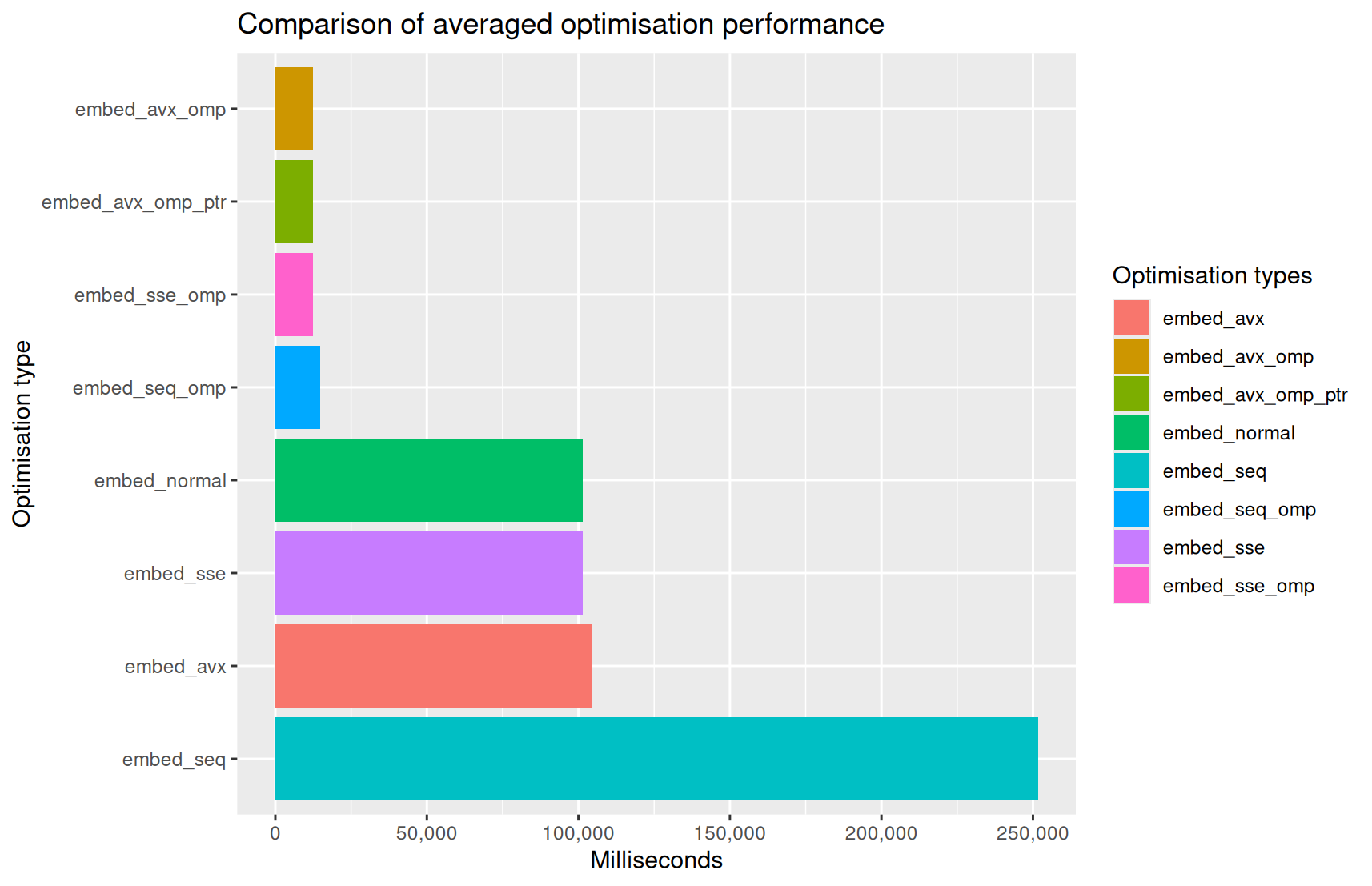
The average number of milliseconds each binary took to complete the task are as follows:
| Binary Type | Count | Mean | Standard Deviation | Minutes | Seconds | Milliseconds | Percentage Reduction | Speedup | |
|---|---|---|---|---|---|---|---|---|---|
| 1 | embed_seq | 38 | 251657.50 | 2159.97 | 4.00 | 11.00 | 657.00 | 0.00 | 1.00 |
| 2 | embed_avx | 38 | 104460.71 | 93.71 | 1.00 | 44.00 | 460.00 | 58.49 | 2.41 |
| 3 | embed_sse | 38 | 101542.39 | 67.85 | 1.00 | 41.00 | 542.00 | 59.65 | 2.48 |
| 4 | embed_normal | 38 | 101538.87 | 83.01 | 1.00 | 41.00 | 538.00 | 59.65 | 2.48 |
| 5 | embed_seq_omp | 38 | 14711.24 | 256.37 | 0.00 | 14.00 | 711.00 | 94.15 | 17.11 |
| 6 | embed_sse_omp | 38 | 12483.68 | 291.65 | 0.00 | 12.00 | 483.00 | 95.04 | 20.16 |
| 7 | embed_avx_omp_ptr | 38 | 12409.84 | 292.90 | 0.00 | 12.00 | 409.00 | 95.07 | 20.28 |
| 8 | embed_avx_omp | 38 | 12362.26 | 48.64 | 0.00 | 12.00 | 362.00 | 95.09 | 20.36 |
The column Mean is the average of the total milliseconds it
took for each binary from the 38 runs. Percentage Reduction is
((A−B)/A) × 100,
where A is time it took for
the sequential version embed_seq (which is the reference)
and B is the binary being
compared took. Similarly, Speedup is A/B.
We can visualise this as follows:
As noted earlier, we do not wish to compare one optimisation against another using specific samples; because, there are statistical variations even between the various runs of the same binary (see the standard deviations above).
What we really want to ascertain is whether a specific optimisation fares better than another on average.
To do this, we first carry out a one-way ANOVA test to confirm that there are indeed statistically significant differences between the various optimisation techniques. Remember that we set the sample size to account for the statistical power etc., which we have described above. Furthermore, the ANOVA test makes certain assumptions about the distribution of the data, and we must confirm these conditions, as discussed in the following.
We run a one-way ANOVA on the 38 × 8 = 304 samples collected, as follows:
df <- read.csv('embedding_results.csv',
        header = TRUE, stringsAsFactors = TRUE)
anova_results <- aov(Milliseconds ~ BinaryType, data = df)
summary(anova_results)
which produces:
             Df    Sum Sq   Mean Sq F value Pr(>F)
BinaryType    7 1.856e+12 2.652e+11  430814 <2e-16 ***
Residuals   296 1.822e+08 6.156e+05
---
Signif. codes:  0 ‘***’ 0.001 ‘**’ 0.01 ‘*’ 0.05 ‘.’ 0.1 ‘ ’ 1
The <2e-16 *** says that there are statistically
significant differences in the performance. So, it is wise to
choose specific optimisations over another. So, which one do we
choose?
Note that the variances for all the groups are not the same, as shown in the table above (variance is standard deviation squared). We should therefore check if the conditions for normality and equality of variance are satisfied, so we can choose a more appropriate test that does not require these conditions.
We can test the normality and equality of variance respectively using Shapiro-Wilk’s and Levene’s tests, as follows:
library(car)
shapiro.test(anova_results$residuals)
leveneTest(Milliseconds ~ BinaryType, data = df)
which produces:
    Shapiro-Wilk normality test

data:  anova_results$residuals
W = 0.50768, p-value < 2.2e-16


Levene's Test for Homogeneity of Variance (center = median)
       Df F value    Pr(>F)
group   7  46.239 < 2.2e-16 ***
      296
---
Signif. codes:  0 ‘***’ 0.001 ‘**’ 0.01 ‘*’ 0.05 ‘.’ 0.1 ‘ ’ 1
Since the null hypothesis for these tests are respectively that the samples are normally distributed and that they have equal variances, the p-value < 2.2e-16 from both these tests say, we can reject both null hypotheses. In other words, we cannot assume normality and equality of variance. We can also see this in the residuals and QQ-plot, as follows:
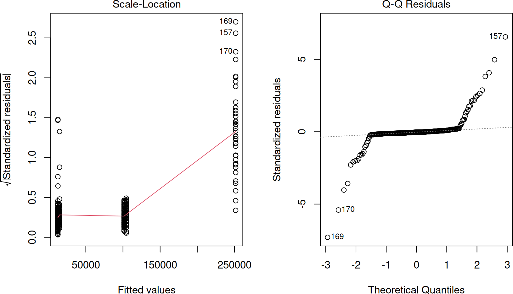
If the data was normally distributed, the QQ-plot (on the right) should not have that many sample deviations from the dashed line. Furthermore, if the variances were equal, the red line on the left should all be horizontal.
Because the condition for equal variance is violated, we need the Welch’s test since a simple one-way ANOVA with an F-test may not be suitable. Even then, we can confirm that for our performance results, there is at least two strategies that have different performances (in both cases the p-value < 2.2e-16).
Without assuming equality of variance, we have:
oneway.test(Milliseconds ~ BinaryType, data = df, var.equal = FALSE)which gives:
    One-way analysis of means (not assuming equal variances)

data:  Milliseconds and BinaryType
F = 9982014, num df = 7.00, denom df = 123.41, p-value < 2.2e-16
With assumption of equal variance, we have:
oneway.test(Milliseconds ~ BinaryType, data = df, var.equal = TRUE)which gives:
    One-way analysis of means

data:  Milliseconds and BinaryType
F = 430814, num df = 7, denom df = 296, p-value < 2.2e-16
Because we violate the normality assumption, we also run the Kruskal-Wallis’ rank sum test, which is a non-parametric test that does not require normality. We do this as follows:
kruskal.test(Milliseconds ~ BinaryType, data = df)which produces:
    Kruskal-Wallis rank sum test

data:  Milliseconds by BinaryType
Kruskal-Wallis chi-squared = 285.78, df = 7, p-value < 2.2e-16
Again, the p-value < 2.2e-16 says that at least two of the strategies have different performances.
To choose a specific optimisation strategy, we must do a posthoc analysis. The one-way ANOVA only tells us that there are differences between the groups. We now need to carry out pairwise comparisons between the strategies. The null hypothesis for each of the pairwise comparisons is that there is no difference between the performances of any two strategies.
Using the Tukey HSD (honestly significant difference) test as follows:
library(multcomp)
posthoc_test <- glht(anova_results, linfct = mcp(BinaryType = "Tukey"))
summary(posthoc_test)
we get:
Simultaneous Tests for General Linear Hypotheses

Multiple Comparisons of Means: Tukey Contrasts


Fit: aov(formula = Milliseconds ~ BinaryType, data = df)

Linear Hypotheses:
                                         Estimate Std. Error   t value Pr(>|t|)
embed_avx_omp - embed_avx == 0         -9.210e+04  1.800e+02  -511.665   <1e-05 ***
embed_avx_omp_ptr - embed_avx == 0     -9.205e+04  1.800e+02  -511.400   <1e-05 ***
embed_normal - embed_avx == 0          -2.922e+03  1.800e+02   -16.233   <1e-05 ***
embed_seq - embed_avx == 0              1.472e+05  1.800e+02   817.770   <1e-05 ***
embed_seq_omp - embed_avx == 0         -8.975e+04  1.800e+02  -498.615   <1e-05 ***
embed_sse - embed_avx == 0             -2.918e+03  1.800e+02   -16.213   <1e-05 ***
embed_sse_omp - embed_avx == 0         -9.198e+04  1.800e+02  -510.990   <1e-05 ***
embed_avx_omp_ptr - embed_avx_omp == 0  4.758e+01  1.800e+02     0.264    1.000
embed_normal - embed_avx_omp == 0       8.918e+04  1.800e+02   495.432   <1e-05 ***
embed_seq - embed_avx_omp == 0          2.393e+05  1.800e+02  1329.435   <1e-05 ***
embed_seq_omp - embed_avx_omp == 0      2.349e+03  1.800e+02    13.050   <1e-05 ***
embed_sse - embed_avx_omp == 0          8.918e+04  1.800e+02   495.452   <1e-05 ***
embed_sse_omp - embed_avx_omp == 0      1.214e+02  1.800e+02     0.675    0.998
embed_normal - embed_avx_omp_ptr == 0   8.913e+04  1.800e+02   495.168   <1e-05 ***
embed_seq - embed_avx_omp_ptr == 0      2.392e+05  1.800e+02  1329.171   <1e-05 ***
embed_seq_omp - embed_avx_omp_ptr == 0  2.301e+03  1.800e+02    12.786   <1e-05 ***
embed_sse - embed_avx_omp_ptr == 0      8.913e+04  1.800e+02   495.187   <1e-05 ***
embed_sse_omp - embed_avx_omp_ptr == 0  7.384e+01  1.800e+02     0.410    1.000
embed_seq - embed_normal == 0           1.501e+05  1.800e+02   834.003   <1e-05 ***
embed_seq_omp - embed_normal == 0      -8.683e+04  1.800e+02  -482.382   <1e-05 ***
embed_sse - embed_normal == 0           3.526e+00  1.800e+02     0.020    1.000
embed_sse_omp - embed_normal == 0      -8.906e+04  1.800e+02  -494.757   <1e-05 ***
embed_seq_omp - embed_seq == 0         -2.369e+05  1.800e+02 -1316.385   <1e-05 ***
embed_sse - embed_seq == 0             -1.501e+05  1.800e+02  -833.984   <1e-05 ***
embed_sse_omp - embed_seq == 0         -2.392e+05  1.800e+02 -1328.760   <1e-05 ***
embed_sse - embed_seq_omp == 0          8.683e+04  1.800e+02   482.402   <1e-05 ***
embed_sse_omp - embed_seq_omp == 0     -2.228e+03  1.800e+02   -12.375   <1e-05 ***
embed_sse_omp - embed_sse == 0         -8.906e+04  1.800e+02  -494.777   <1e-05 ***
---
Signif. codes:  0 ‘***’ 0.001 ‘**’ 0.01 ‘*’ 0.05 ‘.’ 0.1 ‘ ’ 1
(Adjusted p values reported -- single-step method)
This says that, except for the following, there are statistically significant differences between the pairs being compared. Now, using the diagram above, all we need to do is choose the optimisation strategy that is faster between the two. The following strategies, however, have no statistically significant difference in performance:
embed_avx_omp_ptr - embed_avx_omp == 0  4.758e+01  1.800e+02     0.264    1.000
embed_sse_omp - embed_avx_omp == 0      1.214e+02  1.800e+02     0.675    0.998
embed_sse_omp - embed_avx_omp_ptr == 0  7.384e+01  1.800e+02     0.410    1.000
embed_sse - embed_normal == 0           3.526e+00  1.800e+02     0.020    1.000
This is expected. The pair (embed_sse,
embed_normal) is likely using the same SSE instruction set
because the compiler is automatically enabling these for
embed_normal. We also notice that there is no difference in
performance from using pointer arithmetic or the counter method.
Finally, the SEE and AVX does not seem to have statistically significant
differences either, which is puzzling since AVX should be twice as fast
(8 items at a time for AVX compared to 4 for SSE). If we look at the
code, we can see that the SIMD optimisation is limited for each token
line by the number of channels, since, we are processing channels for
each token separately. I believe that the overhead of using AVX for the
limited size of the channels is overshadowing the improvements
gained.
We generate multiple binaries by enabling and disabling compile flags that affect the instructions used. These are:
CC=gcc
CFLAGS=-std=gnu99 -O3 -ffast-math

default: all

embed_normal: embedding.c
    ${CC} ${CFLAGS} -o embed_normal embedding.c

embed_seq: embedding.c
    ${CC} ${CFLAGS} -mno-sse -mno-sse3 -mno-sse4 -mno-avx -mno-avx2 -o embed_seq embedding.c

embed_seq_omp: embedding.c
    ${CC} ${CFLAGS} -mno-sse -mno-sse3 -mno-sse4 -mno-avx -mno-avx2 -fopenmp -o embed_seq_omp embedding.c

embed_sse: embedding.c
    ${CC} ${CFLAGS} -msse -msse3 -msse4 -mno-avx -mno-avx2 -o embed_sse embedding.c

embed_sse_omp: embedding.c
    ${CC} ${CFLAGS} -msse -msse3 -msse4 -mno-avx -mno-avx2 -fopenmp -o embed_sse_omp embedding.c

embed_avx: embedding.c
    ${CC} ${CFLAGS} -msse -msse3 -msse4 -mavx -mavx2 -o embed_avx embedding.c

embed_avx_omp: embedding.c
    ${CC} ${CFLAGS} -msse -msse3 -msse4 -mavx -mavx2 -fopenmp -o embed_avx_omp embedding.c

embed_avx_omp_ptr: embedding.c
    ${CC} ${CFLAGS} -DUSE_POINTER_ARITHMETIC -msse -msse3 -msse4 -mavx -mavx2 -fopenmp -o embed_avx_omp_ptr embedding.c

all: embed_normal embed_seq embed_seq_omp embed_sse embed_sse_omp embed_avx embed_avx_omp embed_avx_omp_ptr